David S. Carter and Ralf von Appen
Abstract
In this study, we combine automated tempo detection, manual adjustments, and statistical analysis in order to examine tempo variability in popular music. Our inspection of 255 Billboard chart-topping singles, supplemented by study of 168 other songs, finds that (1) songs speed up and slow down following several distinct paradigms; (2) measurements of tempo variability can be used to determine with a fair degree of certainty whether a song was recorded with sequenced drums, with a human drummer playing to a click track, or with a drummer playing without a click; and (3) there was a steep decline in tempo variability from 1979 on, largely attributable to increasing use of click tracks and sequencing. We show the value of our method both for study of large-scale trends and for close reading of individual songs.
View PDF
Return to Volume 38
Keywords and Phrases: tempo, ritardando, popular music, click track, drum machine, sequencer, drumming, music technology
1. Introduction
Tempo1 variability—changes in the speed of the tactus—has long been a part of popular music. Just as in common-practice art music (Demos et al. 2020; Demos, Lisboa, and Chaffin 2016) and jazz (Collier and Collier 1994), it can enhance expressivity and create subtle shifts in energy. Such variability can be easily discernible or much more subtle. A tempo shift is a deliberate and discrete change of tempo like those in the Beatles’ “A Day in the Life” or Queen’s “Bohemian Rhapsody,” usually coinciding with the start of a new section (Condit-Schultz and Clark 2024, 5). If the shift is large, then it is easy to identify and describe. But the subtle, continuous tempo variation in music performed and recorded without timekeeping assistance presents more analytical challenges. This variation can constitute small fluctuations up and down or can consist of gradual motion in one direction, with the latter comprising tempo drift (Dahl and Grandqvist 2003, 595).2 Tempo drift is continuous, gradual, more likely to occur withina formal section, and often unintentional. As with microtiming deviations, such changes need not be knowingly carried out by the performer or consciously perceived by the listener in order to have an effect (see Benadon 2006, 95). In this essay we present our method for analyzing tempo variability—both shifts and drift—and apply it to explore this aspect of popular music in singles charting between 1966 and 1995.
Previous analysis of commercial recordings provides a foundation for our research. There has been a good deal of analysis of microtiming in commercial jazz recordings (see, e.g., Friberg and Sundström 2002), and a few researchers in the last fifteen years have attempted to use automatic onset detection in order to measure tempo variability in mainstream pop and rock. Robert J. Ellis et al. (2014) developed an algorithm to analyze the Million Song Dataset for tempo stability, seeking to quickly identify tracks that would be sufficiently stable to aid rehabilitative physical exercise. Stephen F. Roessner (2017), on the other hand, sought to examine historical trends, employing the MIRtempo function in the MATLAB-based MIRtoolbox to measure tempo variability in all 1,098 Billboard number-one hits from 1955 to 2015.3 Nathaniel Condit-Schultz and Beach Clark (2024) examined trends in tempo variability in popular and classical music by analyzing 45,012 music recordings between 1920 and 2020 in the Spotify/Echo Nest library. But as they note themselves, the measurements of beat placement in the Spotify library include many errors and are not reliable (2024, 5, 8–9). A basic problem is that beat detection and tempo estimation algorithms have significant problems with music that lacks regular percussive attacks or that contains ritardandi, accelerandi, or rubato passages (Müller 2021, 311–312).4 Condit-Schultz and Clark (2024, 22) also described their efforts to create a method to determine whether a click track was used but concluded that this method was unreliable.5
In a prior study (Carter and von Appen 2025, 125–134), we introduced a method for examining tempo variability that built upon the previous work of Roessner and Condit-Schultz and Clark but that involved more close listening and manual adjustments to provide greater accuracy and detail. In the present study we expand this method, as explained in Section 2 below, to examine tempo variability in 423 popular songs.6 We analyzed these using automatic tempo map creation in Melodyne, making manual adjustments in order to correct errors by the algorithm. These tempo maps allowed for calculating the coefficient of variation (CV, also known as the relative standard deviation), generating a single number for tempo variability for a song. We supplemented this measurement by using the normalized pairwise variability index (nPVI) and median pairwise calculation (MnPC) in order to determine the average and median size of tempo changes from measure to measure in a recording.
In Section 3 we use tempo CV, nPVI, visual review of tempo maps, and listening in order to identify common patterns of tempo variability. Specifically, we discuss (1) large tempo shifts, (2) internal ritardandi and short-range accelerandi, (3) intros and outros, (4) slightly different tempi for different formal sections, and (5) long-range tempo changes. In Section 4, we explain how CV and MnPCs can be used to numerically distinguish between songs that include sequenced drums, those that were recorded to a click track, and those where the drummer played without a click. In two case studies of songs dating from the time period when click tracks began to be regularly used, we show how our tools can be applied to the analysis of individual recordings. We first examine Bette Midler’s “The Rose” in Section 5, then turn to Gloria Gaynor’s “I Will Survive” in Section 6. In Section 7, we use statistical analysis of our Billboard tempo corpus to examine historical changes in tempo variability. A combination of studying the historical record and careful examination of the recordings themselves confirms that click tracks were the norm in mainstream pop and rock by 1979, with drum machines and sequencing the rule by 1986.
2. Corpora and Methodology
In order to understand how tempo variability in top Billboard hits changed over time, we created two corpora, one to identify diachronic norms and tendencies and the other to develop our method and explore particular technologies. The first corpus, seen in Appendix Table 1 with year-end chart ranking, mean tempo, and tempo variability measurements, consists of the top fifteen singles of the Billboard Hot 100 year-end chart of every even-numbered year between 1966 and 1995.7 We focused on this period because it seemed to encompass the most significant change. We later filled in two additional years within the studied time period—1979 and 1995—in order to include more detail for particularly crucial time spans (see Section 7 below). Thus, the Billboard year-end corpus (hereinafter “the Billboard tempo corpus”) contains 255 recordings. This collection was our primary corpus and is the basis of our statistical analysis.8 We analyzed a second hand-picked sample of 168 recordings in order to get a better idea of the coefficient of variation values associated with the use of different technologies like drum machines, sequencing, click tracks, and loops, as well as to better understand the range of values associated with songs recorded without the use of such technologies. This second corpus (“the supplemental corpus”), seen in Appendix Table 2 with mean tempo and tempo variability measurements for each recording, consists of songs dating between 1935 and 2024 from a variety of genres such as blues, rock, punk, disco, metal, and funk. We did not use this second corpus to calculate comparative statistics because it was not systematically generated.9
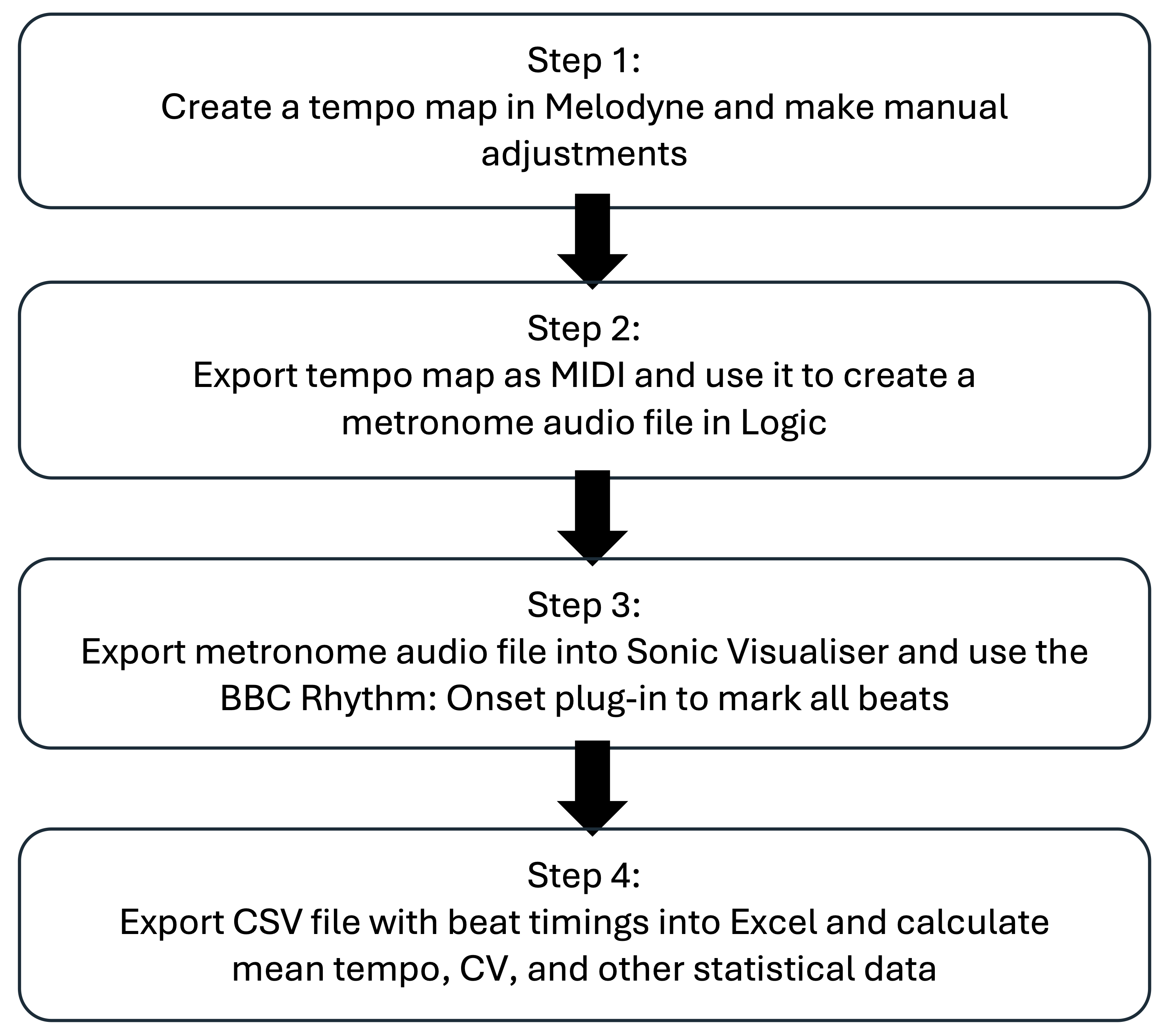
In developing our method, we took advantage of modern automatic tempo detection technology and combined it with manual corrections based on listening. We both (1) created accurate tempo maps of individual songs that allowed for the visual assessment of common shapes and (2) used those maps in order to evaluate tempo variability numerically. Figure 1 shows our workflow. For each song, we began by using Celemony’s Melodyne 5 Studio, an audio editing and analysis application, to generate tempo maps, examples of which can be seen in Section 3 below. These maps allow one to view how the tempo in a track changes over time, showing both large tempo shifts and subtle drift. Melodyne automatically detects note onsets in order to create these maps.10 In songs with consistent drums or percussion and a fairly steady beat, Melodyne’s “Assign Tempo” tool will detect attacks consistently with their perceptual attack times (the instant when a listener would perceive the attack as occurring) and do so in a much more efficient and uniform manner than an analyst annotating each attack individually.
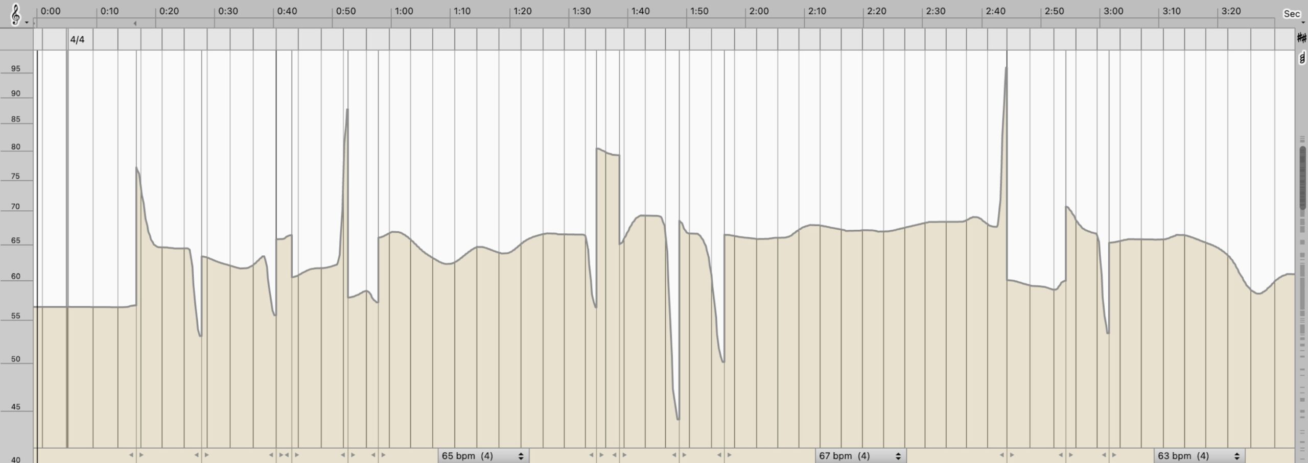
While Melodyne’s automatic beat detection provides an indispensable first step, in many cases it was necessary to manually enter the correct time signature, adjust the detected pulse by doubling or halving it to correct octave errors (see Schreiber 2020, 29),11 or make adjustments with the software’s Tool for Quantized Movement to align the map with the audio. Songs without drums or percussion or with significant ritardandi or accelerandi required more manual adjustments. Examples 1a and 1b show the automatically generated tempo map of Bette Midler’s “The Rose” as well as the same map after we made manual adjustments. This song is exceptional in terms of the amount of adjustment that needed to be made in Melodyne, owing to the lack of drums and the presence of ritardandi at multiple cadences. It was necessary to adjust the position of several beats in the tempo map with Melodyne’s Tool for Quantized Movement in order to match the sounding beat structure. A major strength of the Melodyne interface is that it allows for easy recognition and correction of beat mapping errors: an analyst can identify inaccuracies by watching the playhead move through the tempo map while the audio sounds and a metronome click follows the map. Quick manual adjustments can then be made so that the beats of the tempo map accurately align with the sounding audio.12 Once an adjustment is implemented, the beats of the tempo map for the rest of the song will typically then align automatically with the audio. Given the limitations of current beat-mapping software, these manual adjustments are essential for creating accurate maps.
In addition to employing Melodyne to create tempo maps that allow for visual assessment of common shapes, we used the maps to compute a number that characterizes the tempo variability of a given recording. Because Melodyne currently can neither create an audio file with tempo map metronome clicks nor generate a text file with the time points of these clicks, it was necessary to also employ Apple’s Logic Pro and the free Sonic Visualiser software to assist with this task. Once we had an accurate tempo map in Melodyne, we exported it as a MIDI file into Logic.13 Using Logic’s metronome, we then created an audio file of just the song’s pulse and imported it into Sonic Visualiser. Within this application we used the BBC Rhythm: Onset plug-in to automatically place annotation markers on each beat of the metronome click. We then exported the annotation layer as a comma-separated values (CSV) file into Excel.
With all of the song data in Excel, we were able to analyze it in a variety of ways. We calculated the local tempo of each set of two consecutive measures in the song, with the local tempi determined by measuring the time differential between the relevant downbeats.14 With this information, we then determined the coefficient of variation in order to measure a song’s overall tempo variability. The coefficient of variation, or CV (also known as the relative standard deviation), divides the standard deviation of all the individual local tempo measurements by the mean tempo of the song as a whole.15 We multiplied the CV by 100 in order to express it as a percentage of the mean. A benefit of using the tempo CV rather than just the standard deviation is that it allows for comparison of tempo variability in recordings with vastly different tempi. Tempo CV values theoretically range between 0 and 100. A CV of 0 would in principle indicate no variation in tempo throughout the song. As a practical matter, however, our method of analysis resulted in a CV calculation of 0.01 for songs with no tempo variability. Example 2 shows a Melodyne tempo map for such a song, Peter Cetera’s “Glory of Love” (1986), with time on the x-axis and tempo on the y-axis. The map in this case is a completely flat line. The highest tempo CV value in the Billboard tempo corpus is 23.15, for Don McLean’s tempo-shifting 1972 number-one hit “American Pie.” The median CV for this corpus is 0.76 and the mean is 1.37. The relatively large difference between these two values reflects how sensitive the measurement is to variability, with values rising significantly over the mean when there are ritardandi, accelerations, or tempo shifts. Tempo CV provides a measurement of the overall amount of tempo variability in a song, though it gives no sense of where in the song that variability takes place or how it is distributed.
We calculated a single CV number for each recording in our two corpora. If a song has multiple clearly distinguishable tempi, as is the case with “American Pie,” it can, however, be helpful to calculate independent CV values for each section. A second value can also be useful if one portion of a recording is much steadier than another. If, for instance, a recording used a click track for part of the song but not the whole song, the tempo CV value for the entire song can obscure the fact that a click was used. Calculating separate CV values for the different portions can help identify the use of the click. In Appendix Table 1 we therefore provide multiple tempo CV calculations for songs that have a closing ritardando and in selected other cases. We also list multiple mean tempo values for songs that have more than one distinct tempo.
Because tempo CV does not account for the ordering of individual tempo values within a recording, we also sought to have a measurement that would be sensitive to their arrangement. We therefore employed additional measurements beyond those used in our prior study of the Rolling Stones (Carter and von Appen 2025, 125–134). A hypothetical “Song A” of sixteen measures where the tempo alternated every two measures between 60 BPM and 120 BPM (Example 3a) would have the same tempo CV (33.33) as a “Song B” of sixteen measures consisting of eight measures of 60 BPM followed by eight measures of 120 BPM (Example 3b). Yet the tempo maps and listening experience for these two songs would be dramatically different. A normalized pairwise variability measurement can provide a numerical indication of how the individual tempo values within a song are ordered. The normalized pairwise variability index (nPVI) gives a sense of the relationship between consecutive tempo measurements throughout a recording. Calculating nPVI requires first determining the difference in tempo values for every set of two adjacent measures in a song,16 normalizing each of these values by dividing them by the average of the two tempo measurements. We multiplied each of these individual normalized ratios by 100 for readability, with the resultant pairwise values known as normalized pairwise calculations, or nPCs (Condit-Schultz 2019, 301):
$$\text{nPC}=100*|T_1-T_2|/((T_1+T_2)/2)$$
All of the nPCs in a song would then be averaged in order to generate the recording’s nPVI, a value between 0 and 200.17 The median nPC, or MnPC, reflects the median of all nPC values for a song (instead of the mean) and can also be of value. MnPCs also theoretically range between 0 and 200.
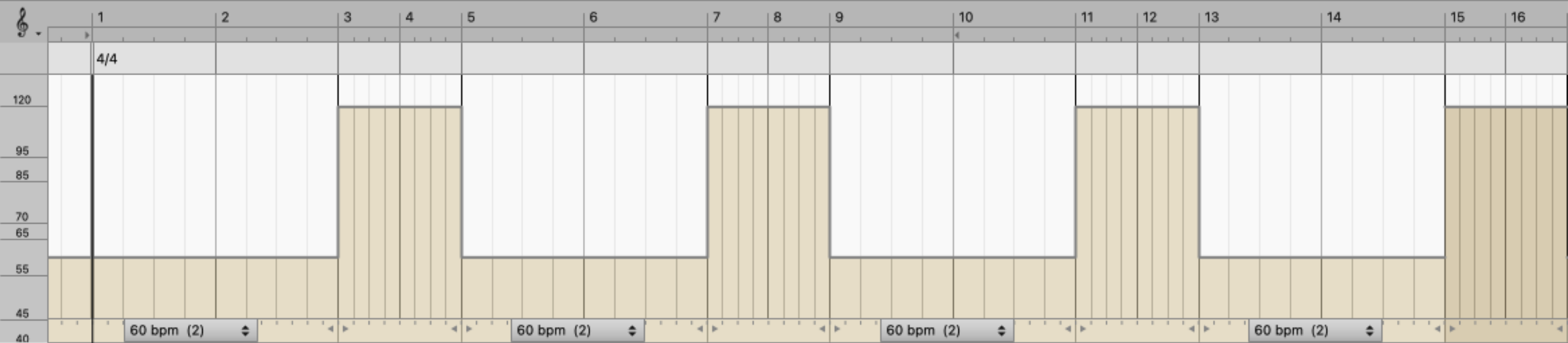
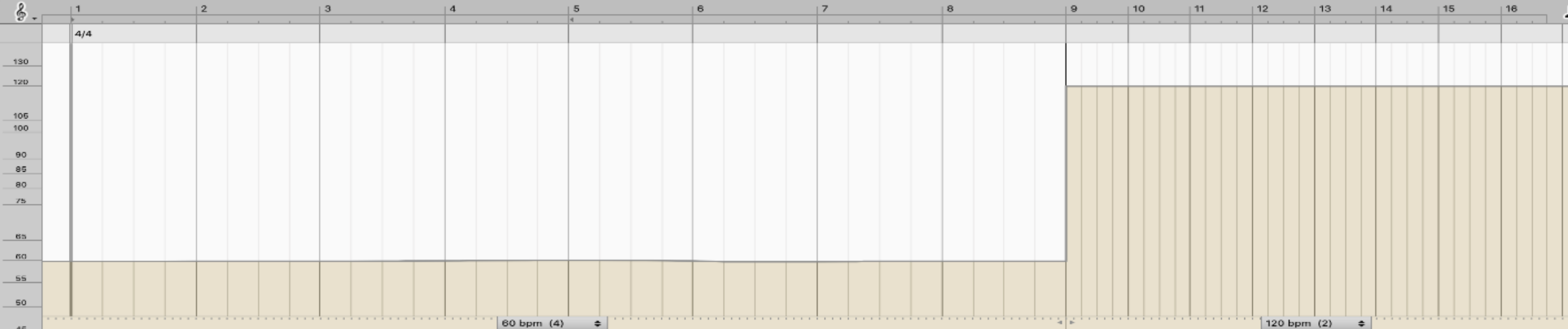
Despite having identical tempo CV (and MnPC) values, the hypothetical Songs A and B would have greatly contrasting nPVI measurements, reflecting their decidedly different structures. Song A, where the tempo values jump back and forth, would have an extremely high nPVI of 31.11. Song B, on the other hand, where similar tempo values were grouped together, would have a much lower nPVI of 4.44. A high nPVI indicates that tempo values move up and down, while a low nPVI indicates that similar tempo values tend to be adjacent to one another. nPVI is thus more sensitive to dramatic ritardandi and shifts than it is to tempo drift: because subtle drift is characterized by very small changes in tempo gradually accumulating, the individual nPCs are small. While the theoretical minimum nPVI value is 0 and maximum is 200, actual values in the Billboard tempo corpus fall within a much narrower range. Within the 255 songs in the collection, the lowest is 0.002 (Peter Cetera’s sequenced “Glory of Love,” 1986, Example 2 above) and the highest is 5.35 (Barbra Streisand’s “The Way We Were,” 1974). The ten highest and ten lowest nPVI values in the Billboard tempo corpus appear in Tables 1a and 1b. The median nPVI value in this corpus is 0.46, with the mean 0.56. MnPC values in the Billboard tempo corpus range between 0 (numerous songs) and 1.41 (Barry Manilow’s “I Write the Songs,” 1976), with 0.32 the median and 0.33 the mean.
| Song | Artist | Year | nPVI |
|---|---|---|---|
| Glory of Love | Peter Cetera | 1986 | 0.002 |
| Wild Night | John Mellencamp and Me’shell Ndegéocello | 1994 | 0.005 |
| What’s Love Got to Do with It | Tina Turner | 1984 | 0.005 |
| I’m Too Sexy | Right Said Fred | 1992 | 0.005 |
| Black or White | Michael Jackson | 1992 | 0.008 |
| This Is How We Do It | Montell Jordan | 1995 | 0.010 |
| All That She Wants | Ace of Base | 1994 | 0.014 |
| All Night Long (All Night) | Lionel Richie | 1984 | 0.015 |
| Never Gonna Give You Up | Rick Astley | 1988 | 0.016 |
| I’ll Remember | Madonna | 1994 | 0.016 |
Table 1a. Lowest nPVI values in the Billboard tempo corpus.
| Song | Artist | Year | nPVI |
| The Way We Were | Barbra Streisand | 1974 | 5.35 |
| Strangers in the Night | Frank Sinatra | 1966 | 4.80 |
| American Pie | Don McLean | 1972 | 3.60 |
| You Light Up My Life | Debby Boone | 1978 | 3.51 |
| Hero | Mariah Carey | 1994 | 2.98 |
| The Rose | Bette Midler | 1980 | 2.71 |
| I Will Survive | Gloria Gaynor | 1979 | 2.52 |
| Say You, Say Me | Lionel Ritchie | 1986 | 1.98 |
| Save the Best for Last | Vanessa Williams | 1982 | 1.97 |
| I Write the Songs | Barry Manilow | 1976 | 1.90 |
Table 1b. Highest nPVI values in the Billboard tempo corpus.
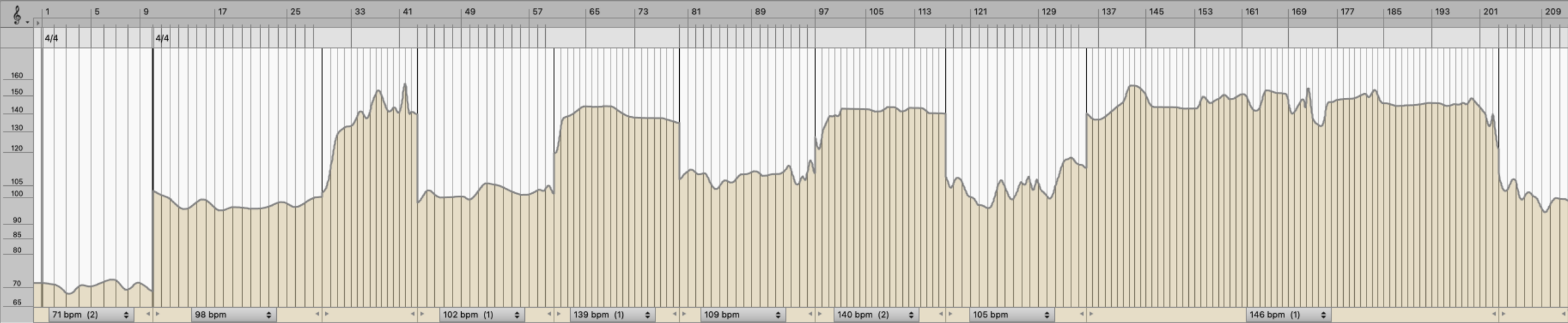
Looking at tempo CV and nPVI values on their own is useful, but it can also be beneficial to consider the ratio between these two numbers: nPVI/CV. This ratio can help differentiate whether tempo variability in a song is the result of tempo shifts, internal ritardandi, or some combination of the two. nPVI/CV ratios in the Billboard tempo corpus range between 0.04 (Donna Summer’s “MacArthur Park,” 1979) and 18.95 (Deniece Williams’s “Let’s Hear It for the Boy,” 1984). The median nPVI/CV is 0.67 and the mean is 1.03. Songs with a clearly audible tempo shift have a nPVI/CV ratio of less than 0.30, while those with at least one internal ritardando have a ratio of 0.30 or greater. Table 2 shows the ten songs in the Billboard tempo corpus with the highest tempo CV values, along with their nPVI and nPVI/CV numbers and whether they have a large tempo shift or an internal ritardando. Songs with a clearly audible tempo shift, such as Diana Ross’s “Love Hangover” (1976), have a lower nPVI/CV ratio because they typically include a more prolonged change of tempo that does not return to the original rate. In such cases, one tempo change results in a large number of contrasting individual tempo values, boosting the tempo CV without incurring any further large nPC values as long as that new tempo is maintained. But songs with internal ritardandi, such as “The Way We Were,” do not remain in the new slower tempo for long and typically return to the previous pulse after the ritardando. This results in a relatively small number of tempo measurements at the differing tempo as well as two high nPCs—at least one when the slowing occurs and another when the original tempo returns. Don McLean’s “American Pie” (1972) has both large tempo shifts and internal ritardandi, and this is reflected in its combination of extremely high CV and nPVI values, while still having a nPVI/CV ratio of less than 0.30.
| Year | Title | Tempo | CV | nPVI | nPVI/CV | Tempo Shift or Internal Rit.? |
|---|---|---|---|---|---|---|
| 1979 | MacArthur Park | 120 | 20.29 | 0.12 | 0.01 | Shift |
| 1976 | Love Hangover | 105 | 14.52 | 0.30 | 0.02 | Shift |
| 1986 | Say You Say Me | 67 | 15.11 | 1.98 | 0.13 | Shift |
| 1972 | American Pie | 123 | 23.15 | 3.60 | 0.16 | Both |
| 1992 | Under the Bridge | 84 | 6.31 | 1.11 | 0.18 | Shift |
| 1970 | Raindrops Keep Fallin’ on My Head | 104 | 9.12 | 1.87 | 0.21 | Both |
| 1978 | You Light Up My Life | 76 | 9.09 | 3.51 | 0.39 | IR |
| 1994 | Hero | 59 | 6.33 | 2.98 | 0.47 | IR |
| 1966 | Strangers in the Night | 90 | 8.98 | 4.80 | 0.53 | IR |
| 1974 | The Way We Were | 66 | 9.76 | 5.35 | 0.55 | IR |
Table 2. The ten songs in the Billboard tempo corpus with the highest CV values, ordered by nPVI/CV ratio.
3. Shifts, Ritardandi, and Shapes
While rock music is usually thought to have a steady tempo (Condit-Schultz and Clark 2024, 2; Temperley 2004, 319), our tempo maps show that tempo variability was used for expressive ends in mainstream popular music in almost half of the corpus examples prior to 1979. This affective or expressive variability can either consciously or unconsciously be used to create contrast or excitement and often reinforces the formal structure of a song. Rhythmic variability, of which tempo variability can be considered a subset, has been recognized as an important vehicle for musical expression, and altering tempo, especially by slowing down, allows performers to express the hierarchical structure of a work (Ashley 2014, 157; Todd 1985, 40, 49).
By using a combination of visual inspection of individual tempo maps, listening, tempo CV, and nPVI, we can identify the most common patterns of such variability. Tempo CV, nPVI, and their ratio (nPVI/CV) allow for numerical assessment of songs and can provide some idea of the shapes and content of tempo variability. But it is also important to adopt non-numerical approaches—to use our eyes and ears—in order to assist in the identification of such patterns. Using a combination of numerical and non-numerical approaches, we found that the most common types of expressive tempo variability in the Billboard tempo corpus include (1) large tempo shifts; (2) reinforcement of structural boundaries by either slowing or anacrustically accelerating when approaching them; (3) employing a different approach in intros and outros than that used in the rest of the song; (4) distinguishing formal sections by using slightly different tempi; and (5) long-term tempo changes across the duration of a song, most commonly an acceleration. Type 2 works primarily at an intermediate level of timing structure, and types 1, 4, and 5 operate at a global level, while type 3 can interact with both intermediate and global levels (Todd 1985, 39–40). A song can contain more than one type.
3.1 Large Tempo Shifts
Large tempo shifts, rare in the Billboard tempo corpus, tend to occur at formal boundaries, creating dramatic contrast between sections. They can either be temporary or permanent and can also be classified by their relative position within a song. Most large tempo shifts in the Billboard tempo corpus are permanent—once the shift occurs, the song stays in the new tempo for the rest of the recording. Some songs have a slower introductory tempo, then switch to a faster pulse that lasts until the end of the recording. Examples include the Red Hot Chili Peppers’ “Under the Bridge” (1992), Diana Ross’s “Love Hangover” (1976), and Donna Summer’s cover of “MacArthur Park” (1979). “Under the Bridge,” for example, starts with a 30-second guitar introduction around 68 BPM that is approximately 15 BPM slower than what follows. B.J. Thomas’s “Raindrops Keep Fallin’ on My Head” (1970; Audio Example 4), on the other hand, ranges between 105 and 110 BPM for most of its duration in a carefree shuffle, then, after a dramatic ritardando, switches to 88 BPM for a short, highly syncopated instrumental outro alternating measures of $$4\atop4$$ and $$5\atop4$$. Lionel Richie’s “Say You, Say Me” (1986), excerpted in Example 5, is unusual in that it has a temporary but large tempo shift for the bridge, taking that section much faster at 98 BPM (almost exactly 1.5 times the previous tempo of 64 BPM) before returning to the original, slower tempo for the remainder of the recording. Large tempo shifts, like internal ritardandi, typically result in a high tempo CV value for a recording, usually above 6.0. But while songs with internal ritardandi have nPVI/CV ratios over 0.30, recordings with large tempo shifts, such as “Love Hangover” and “Under the Bridge,” typically have ratios less than 0.30. In both of these songs the nPVI remains relatively low because there are only one or two high (>10) nPC values, occurring when the tempo shift occurs in the first part of the recording.
3.2 Internal Ritardandi and Short-Range Accelerandi
In the songs we examined, a ritardando is typically a large but relatively brief dip in tempo at a cadence.18 Previous scholarship has addressed the use of rubato, ritardandi, and accelerandi in classical and jazz repertoire (Ashley 2002; Fabian 2014; Friedman 2018). This research shows that performers tend to slow down at structural boundaries (Fabian 2014, 72; Repp 1998, 1086; Repp 1992, 2553) and that tempo variability usually reflects the structure of a work (Todd 1985, 40, 49). Performers of nineteenth-century Romantic repertoire tend to slow at structural boundaries to an extent proportional to the importance of the boundary (Repp 1992, 2553). The same is true in some popular songs, especially ballads. Ritardandi can either occur internally within a song, usually followed by a rapid return to the previous tempo, or they can occur at the end of a recording. Songs with internal ritardandi usually have a closing ritardando as well.
Internal ritardandi tend to result in high tempo CV and nPVI values, with nPVI/CV ratios of 0.30 or greater. Examples include Frank Sinatra’s “Strangers in the Night” (1966, CV = 8.98, nPVI/CV = 0.53) and Bette Midler’s “The Rose” (1980, CV = 5.93, nPVI/CV = 0.51, Example 1b above; see Section 5 below). The tempo maps of “Strangers in the Night” in Example 6 and Video Example 6 show how the pace drops from 88–90 BPM to nearly a halt each time Sinatra reaches the half cadence at the end of the bridge with “a warm, embracing dance away.” In each case there is a subsequent switch back to the prior tempo, further enlarging the nPVI. These ritardandi are essential features that convey the song’s structure and that Sinatra still used in live performances decades later. In the Billboard tempo corpus, recordings with strong ritardandi at internal structural boundaries are relatively rare, but, in addition to “Strangers in the Night” and “The Rose,” include the ballads “The Way We Were” (Barbra Streisand, 1974), “You Light Up My Life” (Debby Boone, 1978), “Three Times a Lady” (the Commodores, 1978), and “The Greatest Love of All” (Whitney Houston, 1986).
A structural boundary such as a cadence can alternatively be approached with a small acceleration, often coinciding with the playing of a drum fill (MacLeod 2024, 19). In Billy Joel’s 1980 AABA-form “It’s Still Rock and Roll to Me,” whose tempo map is seen in Example 7, the largest bumps in the graph come at the ends of the A and B sections. These slight accelerations create anticipation for the start of the next section. Video Example 7 contains an excerpt.
3.3 Intros and Outros
In our corpora, expressive variability occurs most frequently at the starts and ends of recordings, outside the song’s core modules (Summach 2012, 40–41). Intros and outros have a transitional function that bridges the gap between the rhythmic irregularity outside the song and the relatively greater tempo stability in the core of the recording. Intros, links, and outros are often considered “inessential” or “secondary” parts of songs (de Clercq 2012, 100–101), yet these are the portions where tempo variability is most likely to occur. Intros, for instance, are sometimes slower or less steady than a song’s main parts. There can be a clearly audible tempo shift at the end of the intro, as discussed in Section 3.1 above and heard in songs such as “Under the Bridge.” Diana Ross’s 1970 cover of “Ain’t No Mountain High Enough” similarly opens with a brief strings-laden intro that is 15 BPM slower than the music that follows. Intros like these often lack a drum kit or at least avoid the use of a snare drum, and the switch to a faster tempo corresponds with a textural increase to a fuller instrumentation. This is the case with the subtle tempo shift at the start of Nirvana’s “Smells Like Teen Spirit” (1991*).19
Intros can also contain a gradual acceleration followed by a leveling off of tempo once the full texture arrives. Such tempo increases can occur as part of a buildup introduction, where elements are added in stages to build the texture (Attas 2015, 278):20 in Metallica’s “Enter Sandman” (1991*), there is a subtle build in tempo from 120.5 to 123.3 BPM over the first ten measures as textural elements are added in stages. Billboard tempo corpus examples of such subtle opening accelerations include the Monkees’ “Last Train to Clarksville” (1966), the Jackson 5’s “I’ll Be There” (1970), and Vanity Fare’s “Hitchin’ a Ride” (1970). Example 8 contains an excerpt from the tempo map of “Hitchin’ a Ride,” showing a subtle, gradual acceleration in the intro from 127 to 133 BPM. Initial accelerations like these can be intentional or unintentional—studies asking individual test subjects to tap steadily have found that linear tempo drift occurs in both directions, measuring between 0.05% and 0.3% per beat (Madison 2001, 415, table 1). This would equate to a potential increase or decrease ranging between 0.96 BPM and 5.76 BPM over the course of four measures of $$4\atop4$$ if starting at a tempo of 120 BPM. In addition, the phenomenon of joint rushing, where an initial acceleration is followed by a subsequent flattening of the tempo curve, has been found to be common in groups of musicians even when they are seeking to keep a steady tempo (Wolf and Knoblich 2022, 1, 4–6, 9).
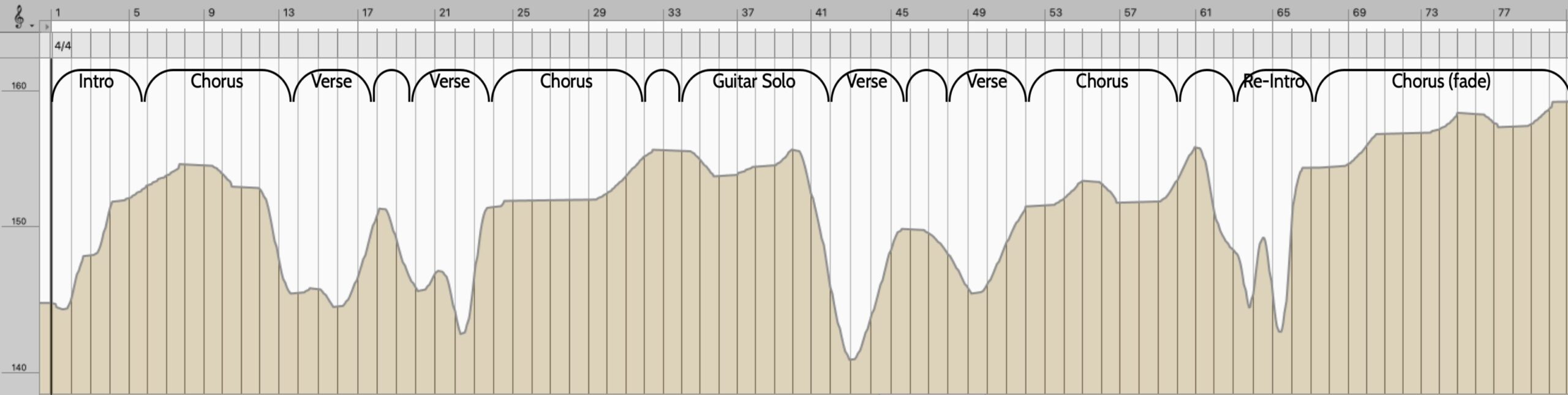
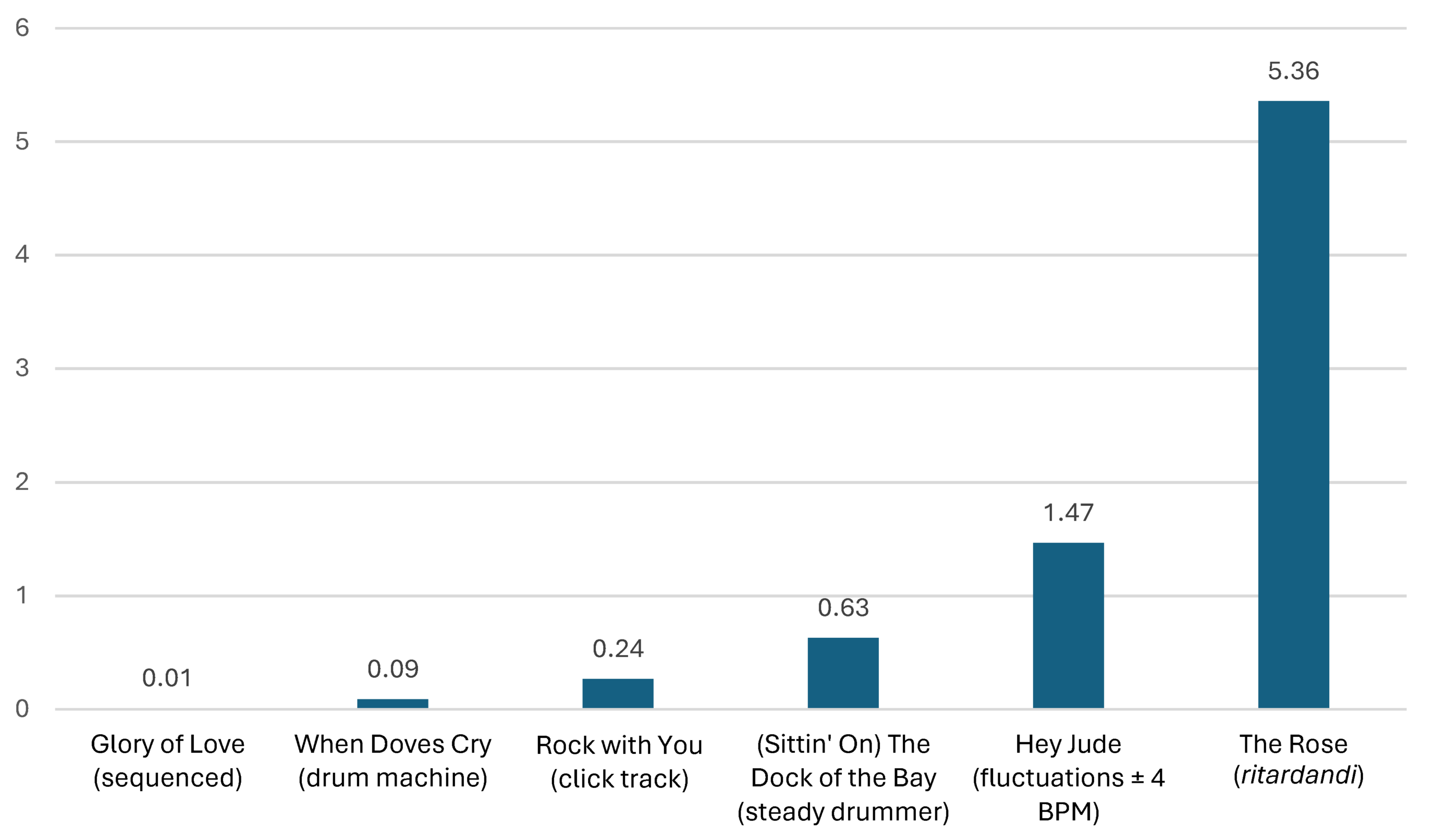
Outros are also frequently a site of tempo variability: occasionally a song will end with an increase in tempo, as in the climactic acceleration leading to a fadeout at the conclusion of The Doors’ “Hello, I Love You” (1968). But closing ritardandi are far more common, occurring in approximately 11% of the Billboard tempo corpus. These tend to occur in ballads, such as Simon & Garfunkel’s “Bridge Over Troubled Water” (1970), Roberta Flack’s “The First Time Ever I Saw Your Face” (1972), and Phil Collins’s “Against All Odds” (1984).21 Songs with just an ending ritardando, but no internal ritardandi, tend to have lower CV values and much lower nPVI values than those with internal ritardandi. While songs with at least one internal ritardando have tempo CV values above 5.25, those with just an ending ritardando have values ranging between 1.5 and 5.25. And while songs with an internal ritardando have nPVI values above 2.5, those with just an ending ritardando have nPVI values ranging between 0.25 and 2. This is in large part because an internal ritardando is typically followed by a relatively quick return to the previous tempo, thus doubling the number of tempo changes and large nPCs. Also, songs with internal ritardandi typically do not make use of sequencing or a click track and usually have more tempo variability throughout their duration than recordings with just an ending ritardando. Bette Midler’s “The Rose” (1980) and Seal’s “Kiss from a Rose” (1995), for instance, have similar tempo CV values, with “The Rose” at 5.36 and “Kiss from a Rose” at 5.66. Yet there is great contrast between their nPVI measurements, with “The Rose” at 2.71 and “Kiss from a Rose” much lower at 1.01. The difference in nPVI comes because “The Rose” has four internal ritardandi, such that the tempo drops four times in the song and then jumps back, followed by a concluding ritardando (Example 1b above). “Kiss from a Rose,” on the other hand, also has an ending ritardando (Audio Example 9), but it has no internal ritardandi and is metronomically steady—recorded with a click track—in the rest of the recording.
3.4 Slightly Different Tempi for Different Formal Sections
While “American Pie” (1972) and “Say You, Say Me” (1986) are rare corpus songs that contain multiple large and clearly audible tempo shifts, it is more common to reinforce a song’s structure by using slightly different tempi for different sections. Artists can accelerate when approaching the chorus, play this section at a slightly faster tempo than the verse, and then return to the slower verse tempo at the start of the second cycle (Hesselink 2023, 137, 142). In the Beach Boys’ “I Get Around” (1964*), for example, the stop-time verses range in tempo between 140 and 145 BPM, while the choruses are roughly 10 BPM faster. Example 10 illustrates how the band consistently follows this pattern and even builds to a tempo high point for the climactic final chorus; Video Example 10 excerpts the start of the song. The Beatles’ “She Loves You” (1964*), Dolly Parton’s “9 to 5” (1980*), and Nirvana’s “Something in the Way” (1991*) speed up for the choruses in a similar fashion.22 If a prechorus is present, tempo alteration can also be used to build tension for the ensuing chorus. Joan Jett & the Blackhearts’ “I Love Rock ‘n Roll” (1982), for example, slows 4.3% during the prechoruses, with this pulling back creating greater anticipation for the chorus, as seen in Example 11. Bridges have the function of creating contrast with preceding material, and a change in tempo can be one way of achieving such contrast. Examples where a contrasting tempo is used for the bridge include Barry Manilow’s “I Write the Songs” (1976) and Paul Revere & the Raiders’ “Kicks” (1966).23 The map in Example 12 shows how the tempo drops 8 BPM for the bridge in “Kicks,” corresponding with a reduction in the instrumental texture.
All of these changes, while relatively subtle, are larger than the 2% minimum for conscious noticeability of tempo change found by Pouliot and Grondin (2005, 394, fig. 3), and even smaller changes can be subliminally perceived (Madison and Merker 2004, 71).Producers have also programmed drum machines or click tracks so that these kinds of slight variations in tempo for different sections are precisely implemented (Hesselink 2023, 141–142; Mynett and Wakefield 2009, 7). In Chris de Burgh’s “The Lady in Red” (1986*), for example, a CR-78 drum machine maintains a steady tempo of 76.1 BPM for the first verse, but the tempo is then increased 1 BPM to 77.1 at the start of the first chorus and remains at that exact pace for the rest of the song.24
3.5 Long-Range Tempo Changes
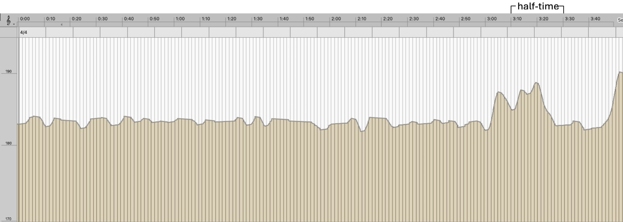
Finally, a recording can have a long-range acceleration across the entire song or a large portion of it. 46% of the pre-1978 songs in the Billboard tempo corpus end at least 3% faster than they begin, and 22% of these (20 out of 90 songs) increase 5% or more. The ten largest accelerations in the corpus, all from prior to 1979, are shown in Table 3a, while Table 3b shows large accelerations from outside the Billboard tempo corpus.25 Example 13 shows how in the Rolling Stones’ “Honky Tonk Women” (1969) the tempo builds continuously over the course of the song from 109 to 127 BPM, a 16% increase; Video Example 13 excerpts the first minute of the song. Given that musicians can detect tempo drift of 0.1% per beat and possibly less (Getty 1975, 5, fig. 1; Kristofferson 1980, 302, fig. 2), the extent of acceleration in “Honky Tonk Women” greatly exceeds the amount that would be detectable by members of the band. This suggests that they either chose to allow tempo drift or intentionally pushed the tempo. As with Sinatra and “Strangers in the Night,” the Stones continued to replicate this approach in live performance to varying degrees.26 A gradual tempo acceleration within a song can thus in some cases be just as essential a part of a composition as lyrics, melody, or harmony.27
Song Artist Year Initial Tempo Final Tempo Tempo Increase The Way We Were Barbra Streisand 1974 64.6 70.9 9.8% Everything Is Beautiful Ray Stevens 1970 106.3 115.6 8.7% Hitchin’ a Ride Vanity Fare 1970 127.0 137.0 7.9% Without You Harry Nilsson 1972 61.2 66.0 7.8% Last Train to Clarksville The Monkees 1966 183.5 197.6 7.7% Seasons in the Sun Terry Jacks 1974 93.6 100.6 7.5% Three Times a Lady Commodores 1978 71.4 76.3 6.9% Let’s Stay Together Al Green 1972 96.7 103.4 6.9% Strangers in the Night Frank Sinatra 1966 89.5 95.6 6.8% Brand New Key Melanie 1972 78.8 83.9 6.5%
Table 3a. The ten recordings in the Billboard tempo corpus with the largest increase from the tempo of the first two bars to that of the last two bars.
| Song | Artist | Year | Initial Tempo | Final Tempo | Tempo Increase |
|---|---|---|---|---|---|
| Can the Circle Be Unbroken (Bye and Bye) | Carter Family | 1935 | 85.6 | 99.8 | 16.6% |
| Honky Tonk Women | The Rolling Stones | 1969 | 109.3 | 126.8 | 16.0% |
| Toro Mata | Celia & Johnny | 1974 | 104.4 | 121.4 | 16.3% |
| Hells Bells | AC/DC | 1980 | 95.7 | 110.8 | 15.7% |
| Purple Haze | Jimi Hendrix Experience | 1967 | 98.7 | 113.2 | 14.7% |
| I’m So Tired | The Beatles | 1968 | 66.9 | 75.6 | 12.9% |
| Train Under Water | Bright Eyes | 2005 | 118 | 132.9 | 12.6% |
| Just Make Love to Me | Muddy Waters | 1954 | 75.7 | 84.9 | 12.2% |
| All Along the Watchtower | Jimi Hendrix Experience | 1968 | 105.4 | 117.4 | 11.4% |
| Babies | Pulp | 1993 | 149.9 | 165.7 | 10.5% |
Table 3b. The ten recordings in the supplemental corpus with the largest increase from the tempo of the first two bars to that of the last two bars.
Decreasing the tempo across the whole of a recording is rare in the Billboard tempo corpus. This finding is consistent with the extensive scholarship noting the tendency of groups of nonmusicians or musicians to accelerate when performing (e.g., Wolf and Knoblich 2022) and reflects the consideration that a gradual decrease in tempo could be deflating in a performance that is aiming to maintain listener attention and create excitement. Table 4 shows the six songs in the Billboard tempo corpus that slow down by at least 3%.28 The comparison here is between the tempo of the first two measures and that of the last two measures, prior to any closing ritardando.
| Title | Artist | Chart Year | Start Tempo | End Tempo | % Change |
|---|---|---|---|---|---|
| My Ding-a-Ling | Chuck Berry | 1972 | 134.5 | 122.0 | -9.3%* |
| Rosanna | Toto | 1982 | 86.4 | 81.6 | -5.6% |
| Let It Be | The Beatles | 1970 | 72.9 | 69.3 | -4.9%* |
| Love Hangover | Diana Ross | 1976 | 117.3 | 111.6 | -4.9%# |
| You Light Up My Life | Debby Boone | 1978 | 80.7 | 77.0 | -4.7%* |
| Hard to Say I’m Sorry | Chicago | 1982 | 74.5 | 72.2 | -3.1%* |
Table 4. Songs in the Billboard tempo corpus that end at least 3% more slowly than they began, even without considering closing ritardandi.
*=A closing ritardando (not counted in the percentage change) further decreases the ending tempo.
#=This gradual slowdown occurs in the up-tempo (majority) disco section of the song (starting at 1:12), after the slower intro.
4. Using Tempo Coefficient of Variation Values to Detect Click Tracks or Sequencing
Our approach can also help identify the presence or absence of tempo-preserving technology in the recording process. Click tracks have largely been a hidden but crucial element of pop music, rarely recognized by consumers and the subject of little scholarship (Théberge 2016, 341). They have “an ambiguous material existence” because they are usually audible only to the drummer through headphones (342). When references to the history of click tracks occur, there is a consistent tendency to be vague about the timing of their ascendance, to date their origins as later than their actual emergence, and to underestimate their pervasiveness in mainstream pop and rock.29 Without solid evidence, it can be difficult to determine whether a click was used in the recording of a given song,30 particularly because artists and producers often seek to hide their use.31 Yet their widespread employment has exerted a powerful influence on the shape of pop and rock.
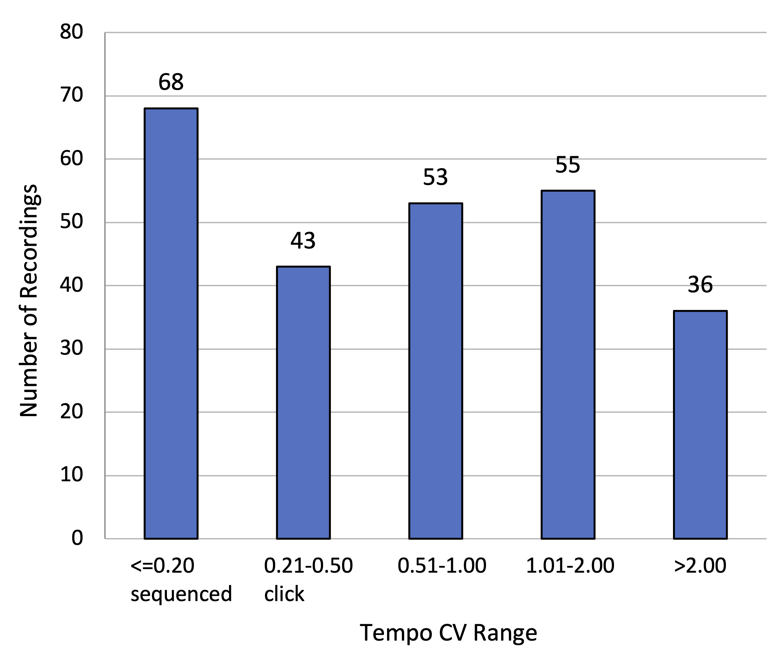
Identifying a song’s tempo CV and median nPC values can provide insight into the probable approach to its recording and aid in analysis. While it can often be hard to come by, in some cases information is publicly available regarding whether a click track was used for a given song.32 Table 5 shows songs known to have been recorded with different timekeeping aids: yellow songs feature a sounding drum machine, sequencing, or tape loop; orange ones feature a human drummer playing to a click track or overdubbing a drum machine; and blue recordings feature a human drummer playing without a click. By calculating the tempo CV values of these songs and others, one can determine which values are associated with which methods. Building on these comparisons, within this section we discuss the CV values associated with (1) the use of sequencing, a sounding drum machine, or a drum loop; (2) recording to a click track or drum machine used as a click; (3) playing steadily but without a click; and (4) having intentional tempo shifts and/or ritardandi. An overview of the number of recordings in the Billboard tempo corpus falling within each of these CV ranges appears in Figure 2, while Figure 3 provides a visual comparison of the tempo CV values of representative songs from each category.
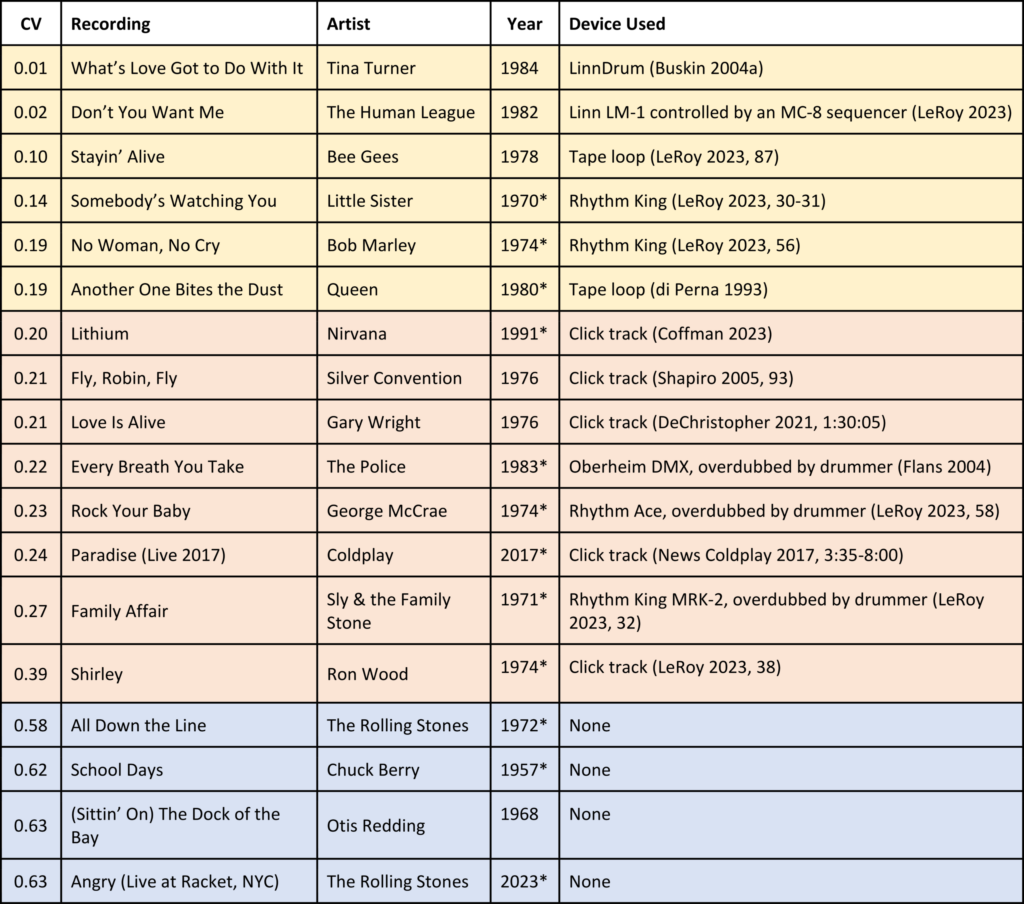
Recordings featuring a tape loop, a sounding drum machine, or (in more recent years) digital quantization tend to have CV values less than 0.2. The Bee Gees’ “Stayin’ Alive” (1978), for instance, used a looped tape recording of a human drummer (CV = 0.10; LeRoy 2023, 87), as did their “More Than a Woman” (1977*, CV = 0.02; LeRoy 2023, 87), Queen’s “Another One Bites the Dust” (1980*, CV = 0.19; di Perna 1993), and Olivia Newton-John’s “Make a Move on Me” (1981*, CV = 0.09; Wikane 2022). The lowest CV values in the Billboard tempo corpus—for songs where the drums (and often other instruments) are fully sequenced—were 0.01, such as for Peter Cetera’s “Glory of Love” (1986; Example 2 above).
Tracks with a human drummer playing to a click or over a drum machine, on the other hand, tend to have values between 0.2 and 0.5, as human drummers inevitably introduce slight variability even when guided by a metronome. For instance, on Gary Wright’s hit “Love Is Alive” (1976, CV = 0.21), Andy Newmark relied on a Rhythm Ace drum machine to keep steady while he played an acoustic drum kit (DeChristopher 2021, 1:30:05). The recording’s median tempo is 98.3 BPM, and the two-measure tempo measurements lie within the relatively narrow range of 97.8 and 98.8 BPM, with the standard deviation 0.20 BPM. On Michael Jackson’s “Rock with You” (1980), drummer John “JR” Robinson played along to a UREI film click (Williams 2023), resulting in a tempo CV of 0.24 (Example 14). The lower end of the click track range, near 0.2, may reflect drummers attempting to stay with a click or drum machine as closely as possible, while the upper end, near 0.5, may reflect a freer approach in which the drummer follows the click but also pushes and pulls against it.33
CV values between 0.5 and 2 are quite possible without timekeeping assistance. There is no evidence that the drummers for Otis Redding or Chuck Berry, producing values around 0.6, used any kind of metronome in their 1950s and 1960s recordings (Table 5). Chic’s “Le Freak” (1979) has a tempo CV of 0.46, with the band’s Nile Rodgers claiming the group never recorded to a click track (Buskin 2005). If true, “Le Freak,” with Tony Thompson, known as “the human metronome” on drums (Shapiro 2005, 87), would represent the lowest CV we found for a track recorded without timekeeping assistance. The lowest CV for a live recording made without timekeeping assistance that we found is 0.63, from the Rolling Stones’ performance of “Angry” at Racket NYC (2023*). The lowest tempo CV values in the Billboard tempo corpus prior to 1976 (the first corpus year in which a song in the top 15 was recorded to a click; see Section 7 below) are Otis Redding’s “(Sittin’ On) The Dock of the Bay” (1968, CV = 0.63), Maria Maldaur’s “Midnight at the Oasis” (1974, CV = 0.64), and Jimmy Ruffin’s “What Becomes of the Brokenhearted” (1966, CV = 0.67). The lowest tempo CV values where no click track or drum machine was used from before 1976 that we found among studio recordings outside of the Billboard tempo corpus are the Rolling Stones’ “All Down the Line” (1972*, CV = 0.58) and “Bitch” (1971*, CV = 0.61). Both the median (0.76) and mean (1.37) CV for the 255 songs in the Billboard tempo corpus fall within this range between 0.5 and 2, where the tempo is fairly steady but no click track was used. While the median of 0.76 indicates that most of the songs in the Billboard tempo corpus did not use a click track, drum machine, or sequencing throughout, the proportion that did increased over time (see Section 7, below).
A tempo CV of 2 or above is indicative of intentional tempo shifts, the use of ritardandi, or a somewhat freer approach to tempo. Recordings with clearly audible tempo shifts, like Don MacLean’s “American Pie” (1972, CV = 23.15) and Lionel Richie’s “Say You, Say Me” (1986, CV = 15.11), can have tempo CV values over 15. Songs with prolonged accelerations can lead to tempo CV values over 10, such as 18.00 for The Velvet Underground’s “Heroin” (1967*) and 10.40 for Dinosaur Jr.’s “Feel the Pain” (1994*). Example 15 shows a tempo map for “Heroin,” which features alternation between slow and fast tempi. Songs with internal ritardandi like “The Rose” (5.36) and “Strangers in the Night” (8.98) also have CV values well over 2.
0.5 works as a general guide when seeking to use tempo CV in order to distinguish songs that used a click track or other timekeeping implement from those that did not, but it is not an unfailing dividing line. There is a good deal of variation in how humans perform with and without click tracks. Additionally, small measurement inaccuracies are possible, and approaches to recording with respect to tempo variability can sometimes be complex. While one might think that songs either used a click track or did not, there are many hybrid cases where a click was used for only part of a song or where a sounding drum machine or sequence was accompanied by human overdubs of drum kit components or percussion.
In cases where sequencing or a click track was used for part but not all of a song, the tempo CV alone may not reveal the use of such an approach. If timekeeping assistance was used for only part of a track, then the tempo CV for the song as a whole will often be outside the usual range indicating such assistance. Individual pairwise measurements, however, have the advantage of being able to suggest from just a few measures whether sequencing or a click track was employed. Typical individual nPCs for a song with sequencing tend to be less than 0.2, while those for a song recorded to a click track tend to range between 0.1 and 0.6. Songs that are steady but not played to a click, such as Wild Cherry’s “Play That Funky Music” (1976, CV = 0.79), may have passages with nPCs resembling those played with a click, but will tend to have many nPCs over 0.6, and perhaps ten or more nPCs of 1.0 or higher over the course of a song. Individual nPCs of 10 or higher are associated with a clearly audible ritardando or tempo change.
The median nPC (MnPC) can supplement tempo CV determinations and can reveal the use of sequencing or a click in some cases where the tempo CV alone does not. MnPC is not quite as reliable as tempo CV as a general tool for determining whether a click track was used, but it can be particularly valuable for identifying instances where sequencing was used for a portion of a recording rather than for the full song. While tempo CV calculations are extremely sensitive to one or two outlier tempo values, MnPC helps identify the recording’s predominant approach. MnPC values of 0.15 and under are associated with sequencing or a loop, while values between 0.15 and 0.30 are associated with use of a click track.34 MnPC works better than nPVI for revealing partial use of timekeeping assistance because outlier nPC values do not affect it.
In some instances where the tempo CV is in a substantially higher range than the MnPC value, the MnPC can reveal the use of a click or sequencing. For example, the Bee Gees’ “You Should Be Dancing” (1976*) has a CV of 0.61, higher than the typical range for recordings using a click. But the MnPC is 0.28, within a range consistent with click use. Bee Gees drummer Dennis Bryon wrote in his memoir that the song was recorded to a click (Bryon 2015, 179), confirming the implication of the MnPC value. It is possible that a click was used for most of the song but not all of it, resulting in the relatively high tempo CV. As another example, Culture Club’s “Karma Chameleon” (1984; Example 16) has a tempo CV of 0.63, higher than the normal range for songs recorded to a click and well outside the typical range for songs with sequenced drums. But the recording is extremely steady for most of its duration and even features five consecutive measures (at 1:38–1:46) where the tempo is exactly 183.546 (nPCs = 0). Yet the last quarter of the song’s duration features significant tempo variability, with acceleration up to 189 BPM by the end of the fadeout. The song’s MnPC of 0.11 lies within the range associated with sequencing. Steve Levine, the producer on the track, revealed in a 2003 interview that the drums for the song did in fact come from a sequenced LinnDrum, yet due to a technical problem the machine accelerated in the latter part of the recording (Inglis 2003). Thus the MnPC reveals the use of sequencing even though the tempo CV does not.
Median nPC values are particularly useful in combination with tempo CV for recognizing instances where a song uses sequencing throughout except for an ending ritardando. These songs have tempo CVs that are relatively high, typically larger than 1.50, but have median nPC values within a range indicating sequencing. Examples where sequencing is used throughout except for an ending ritardando include Mariah Carey’s “Vision of Love” (1990, CV = 4.11, MnPC = 0.06), George Michael’s “One More Try” (1988, CV = 2.04, MnPC = 0.10), Atlantic Starr’s “Secret Lovers” (1986, CV = 1.56, MnPC = 0.05), and All-4-One’s “I Swear” (1994, CV = 3.08, MnPC = 0.05). Songs that seem to use a click track throughout except for an ending ritardando include Eric Clapton’s “Tears in Heaven” (1992; CV = 1.84, 0.26 without rit.; MnPC = 0.35); Mr. Big’s “To Be with You” (1992; CV = 1.66; 0.29 without rit.; MnPC = 0.43); Bryan Adams, Rod Stewart and Sting’s “All for Love” (1994; CV = 2.12, 0.38 without rit.; MnPC = 0.36); and Seal’s “Kiss from a Rose” (1995; CV = 5.66; 0.30 without rit.; MnPC = 0.37). Each of these latter four songs has an MnPC value in an ambiguous range (0.32–0.43), where click use is possible but not certain, but in each case calculation of a CV value without the ending ritardando strongly suggests click track use. These recordings achieve both the idealized steadiness that comes with playing to a click but also allude to earlier musical traditions that would create a sense of finality by slowing at the end. Drummers have discussed how, in the studio, they sometimes would start a song playing to a click, but at a certain point during the take, the producer would turn it off and let the musicians continue to the end without it (Bryon 2015, 162–163; Hesselink 2023, 136–137).35
In addition to instances where sequencing or a click track was used for only part of a track, another kind of hybrid situation can occur when a human drummer overdubs a sounding drum machine. Billy Idol’s 1983 album Rebel Yell is often credited as having ushered in the adoption of hybrid approaches, with combinations of drum machines and live overdubs (Hesselink 2023, 131). But there are examples of this happening as far back as Sly and the Family Stone’s “Family Affair” (1971*), which combined a sounding Maestro Rhythm King MRK-2 with overdubbed human drumming (LeRoy 2023, 29–32; Heath 2017).36 Drum parts in Anglo-American popular music between 1975 and 1995 frequently employed such a hybrid approach (Hesselink 2023, 131–132, 145–146). It was common, for instance, to use a sounding drum machine for the kick and/or snare but for a human drummer to overdub hi-hats, toms, and/or crash cymbals (Hesselink 2023, 132). The Police’s “Every Breath You Take” (1983*), for example, used an Oberheim DMX drum machine for the kick but had snare, hi-hat, and cymbals overdubbed by drummer Stewart Copeland (Buskin 2004b). The tempo CV and MnPC values for songs with both a sounding drum machine and substantial human overdubs tend to be in or near the range typical for a click track. “Family Affair,” for instance, has a tempo CV of 0.27 and an MnPC of 0.38, while “Every Breath You Take” has a tempo CV of 0.22 and an MnPC of 0.21.
5. Case Study #1: Tempo Variability Analysis of Better Midler’s “The Rose”
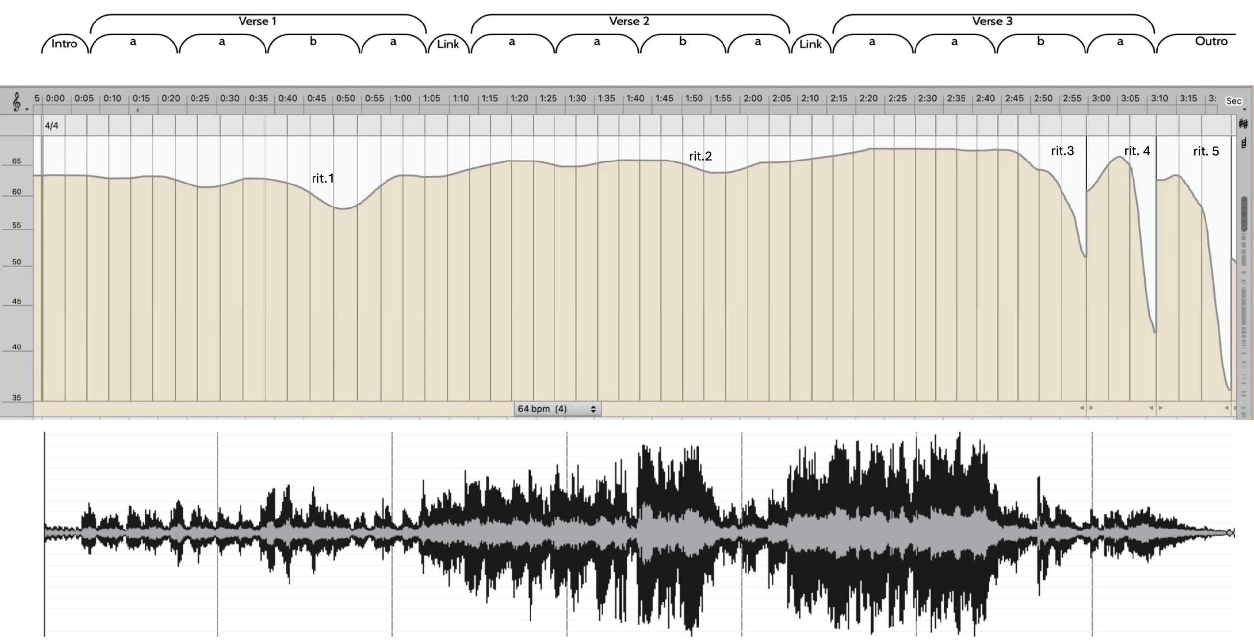
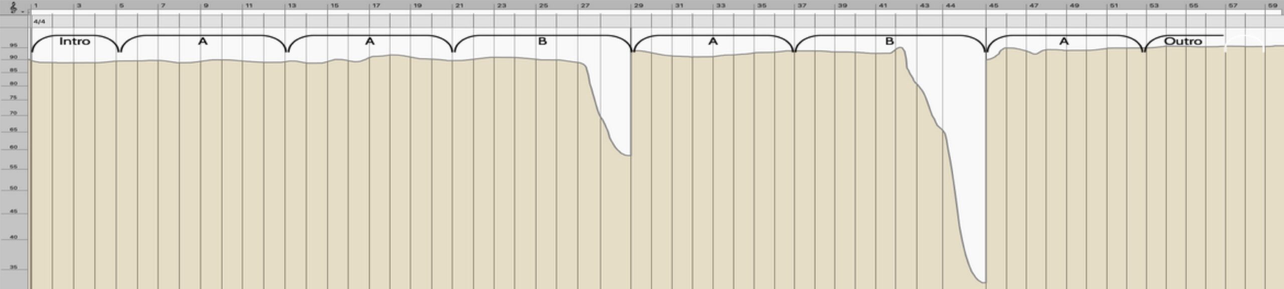
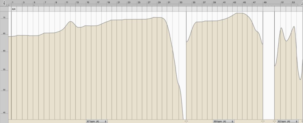
A closer look at Bette Midler’s “The Rose,” the #10 song of 1980, illustrates how examination of patterns of tempo variability and tempo CV analysis can provide insight into particular recordings. “The Rose” was released on the film soundtrack album of the same name in late 1979, the year that tempo invariability came to be the norm on the pop charts (see Section 7 below), yet its CV of 5.36 and MnPC of 0.95 indicate that it was not recorded to a click track and reflect its use of ritardandi in several spots. Example 1b (in Section 2 above) shows the tempo map of the recording. The song, in strophic form, consists primarily of three fifteen-measure aaba verses separated by two-measure links. The tempo trajectory of “The Rose” closely mirrors its textural arc, building from 63 BPM to a high point of 68 BPM, an increase of 8%. The first verse, starting at 63 BPM, begins with solo piano and vocalist; the second verse adds a vocal harmony and additional instrumentation; and the third adds still more vocal harmonies and additional orchestral instrumentation, with the tempo reaching its high point of 68 BPM at 2:22 to 2:37. The fullest texture, with its chorus-like vocals and soaring brass lines, continues until 2:42, after which the harmony vocals and orchestra are reduced. As the texture diminishes in stages in the final 45 seconds of the track, the tempo also slows and the song ends with a succession of ritardandi.
These ending ritardandi are the last of a total of five in the recording, notated in Example 17. These all occur at cadences, contributing strongly to the song’s temporal shape and resulting in a relatively high tempo CV of 5.36 for the track. The song’s nPVI/CV ratio of 0.51 is within the range associated with internal ritardandi (greater than 0.30). Each of these ritardandi prolongs a dominant harmony, thereby building anticipation of resolution for the listener.37 Three of these ritardandi (the first three in Example 1b and Example 17) occur at the ends of the b sections of the three verses, with this b phrase in each case the only one that ends on a half cadence. Of these three ritardandi, the first and the third are the deepest tempo drops and also the half cadences with the thinnest texture. Beyond these three, there are two additional instances of cadential slowing at the end of the song that contribute to a sense of closure. The first of these final two instances occurs at 3:11, with the lead vocalist and solo piano lingering on the dominant harmony of the last authentic cadence involving the vocal. The subsequent final ritardando of the song brings the tempo of the recording to its lowest point (nPC of 27.46, the largest in the recording). Here, the solo piano lingers again on the dominant before resolving to tonic on the final downbeat.
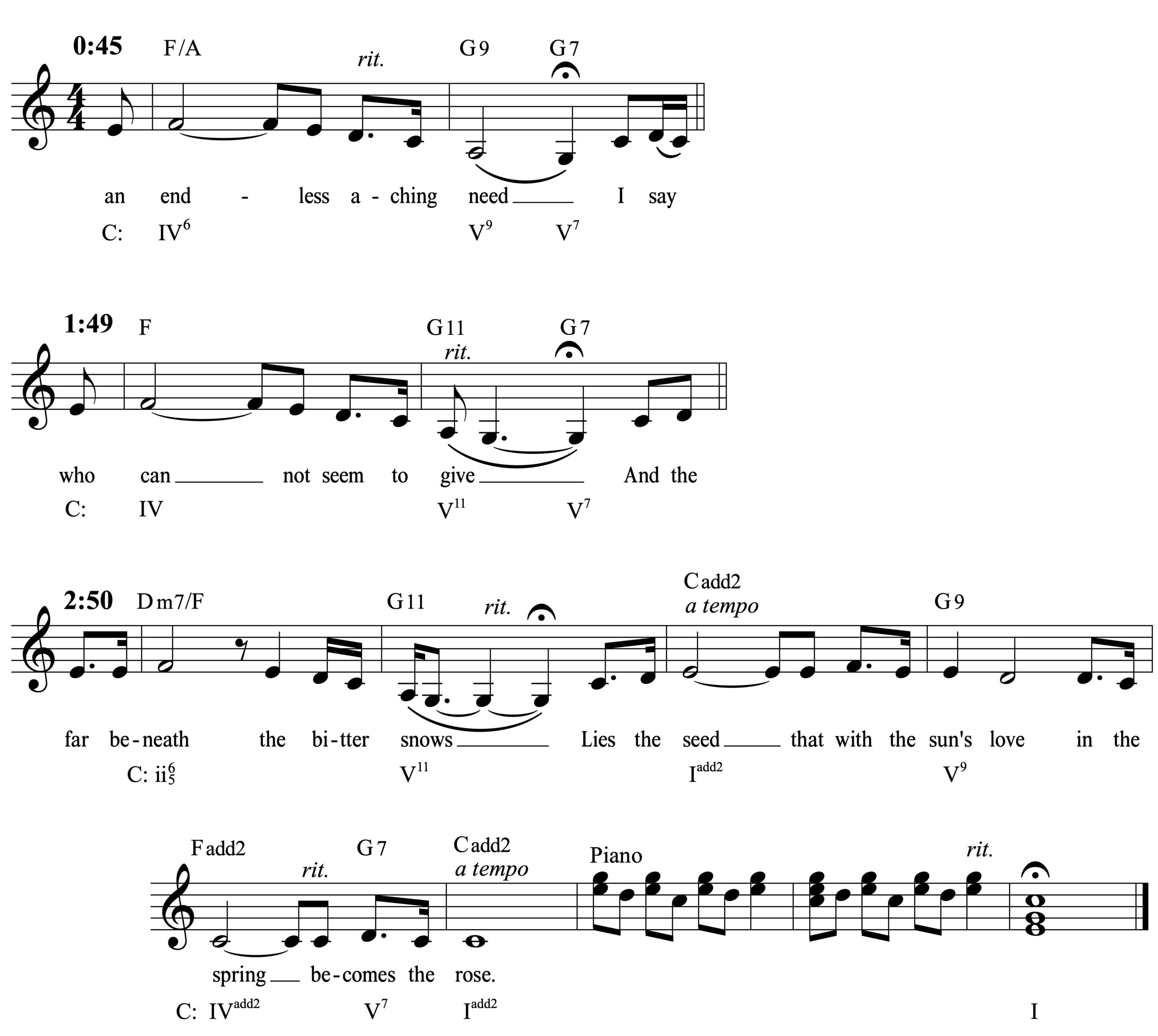
Audio Example 17. The five significant ritardandi in Bette Midler’s “The Rose.”
These five ritardandi contribute greatly to the high tempo CV value in “The Rose” (CV = 5.36), but the long-range acceleration through the first two and a half verses is also an important factor. If we remove the five biggest two-measure outliers from the mean tempo of 63.6 BPM, the CV would be 3.10, still significantly higher than the median tempo CV of 0.65 for its year on the charts, 1980. The approach to tempo in “The Rose” follows a decidedly different model than the one that had come to dominate the top of the Billboard Hot 100 by the time of its release and can be heard as a reaction against the nearly perfect steadiness of click tracks in disco. The song is a throwback to an earlier time period and connects with Tin Pan Alley, ballads in nineteenth-century American popular song, and the common-practice art music tradition. It adheres to a model in which tempo is highly responsive to texture and harmony and is used expressively as a means of reinforcing the structure of the song (Todd 1985, 40, 49).
6. Case Study #2: Tempo Variability Analysis of Gloria Gaynor’s “I Will Survive”
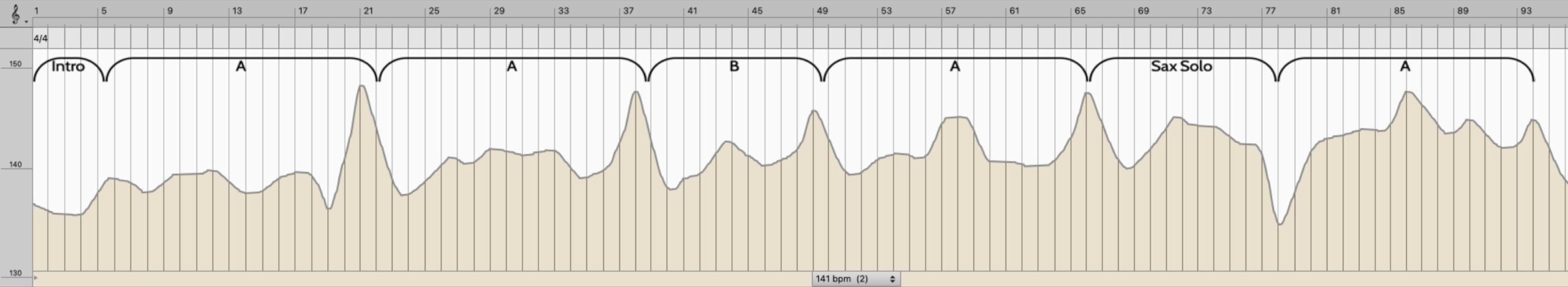
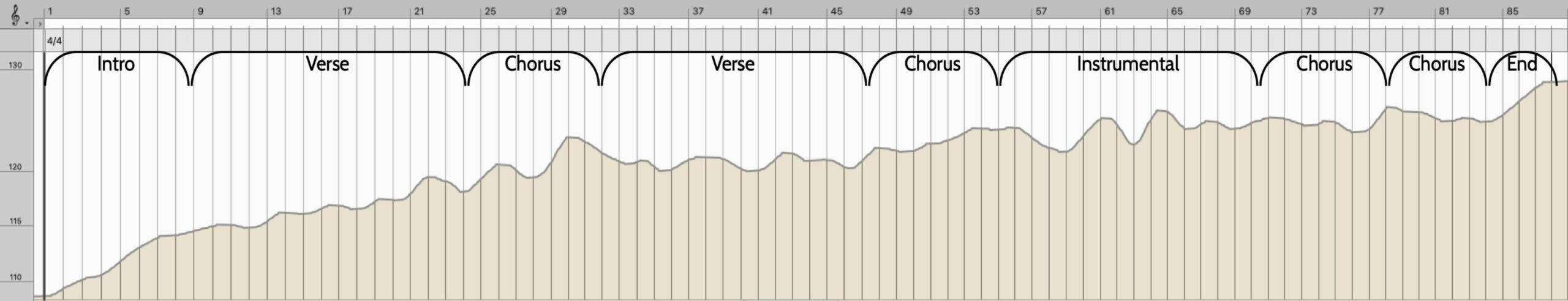
Gloria Gaynor’s “I Will Survive” (seven-inch single version, released in October 1978 and the #6 song of 1979) provides a contrasting example of tempo variability, as it made use of a click track or a drum machine functioning as a click in the recording process but maintained elements of expressive tempo shaping. Example 18 shows that the vast majority of the track’s Melodyne tempo map forms a nearly straight line, reflecting a constant tempo of 116 BPM. Yet the map shows some variability at the start of the song as well as a large dip at 2:32–2:38. The recording illustrates how metronomic technology, which is often concealed as a click that is inaudible to the listener, can be further hidden by gestures that seemingly are at odds with the use of such technology. The song is a combination of near-perfect steadiness and moments of expressive tempo variability that connect with prior popular music practices.
The tempo CV for “I Will Survive” as a whole is 0.38. Tempo CV can provide an overall sense of the variability of a recording, but calculating the MnPC (0.11 in this case) and examining the song in more detail can provide a better understanding of its approach. The tempo CV value for “I Will Survive” suggests the use of a click track in recording, which drummer James Gadson has confirmed in an interview (Amendola 2007, 117). The MnPC value is slightly below the minimum threshold of 0.15 typically associated with a click track, indicating exceptionally steady playing. These CV and MnPC calculations, however, by necessity exclude two moments in the song where there is no detectable meter. The first comes in the song’s opening, with the piano freely arpeggiating a dominant ninth chord that prepares the listener for the A minor tonic beneath the vocalist’s first entrance. The second free moment is an echo of this initial arpeggiation that comes toward the end of the song, at the 2:32–2:38 span that is represented by the large dip in the tempo map in Example 18. Here, as seen in Example 19, there is another teasing lingering on dominant harmony and an arpeggiation (this time by the harp rather than the piano) that prepares the listener for the return of tonic and another verse. The music virtually comes to a complete halt here; the lead vocalist’s exclamation and the brief movement in the strings provide perhaps a suggestion of a very free, slow pulse in the range of 30–60 BPM, but there are no drums and little real sense of meter.38 Yet this pause, while sounding improvisatory and free, can be considered only a simulated escape from the confines of a steady pulse, since the time of the dropout is equivalent to three almost perfectly timed measures at the click track tempo of 116 BPM. It is therefore likely that the producers left the click track running, with this brief span acting as a departure from the prevailing temporal structure for listeners while maintaining temporal continuity for the performers. Through a kind of sleight of hand, the producers create a sense of expressive freedom in a track that is to a large extent grounded in hidden mechanical precision.39
In addition to these two seemingly free moments in the recording, there is another portion with more limited rhythmic freedom—the vocal introduction. This introduction, like the pause on the dominant later in the recording, connects with earlier traditions of popular music, including the often rhythmically free sectional verses that introduced Tin Pan Alley songs. As seen on the far left of Example 18, there is significant tempo fluctuation for the first eight measures after the initial piano arpeggio. The tempo in this region ranges between 112 and 122 BPM, with nPCs ranging between 0.21 and 3.63. This degree of tempo fluctuation strongly suggests that no click track was used during this portion. The drums in this passage play cymbal rolls rather than any kind of regular beat, and the guitar follows Gaynor’s relatively free interpretation of the melody even as the bass lands on each of her downbeats. Once the click track is turned on and the four-on-the-floor drum pattern commences, comparing the eighth and ninth measures gives an nPC of 0.11, the first nPC value lower than 0.2. Most of the remaining nPCs in the song are below this threshold. This freer intro, followed by a metronomically steady disco beat for nearly the entire remainder of the recording, echoes the opening of Donna Summer’s “MacArthur Park” (1979), released two months earlier in August 1978.
If we exclude the opening arpeggiation and later fermata as well as the vocal introduction, then the CV value for the recording would be 0.16, which is close to the typical range for a click track (0.2–0.5) though slightly below it. It is consistent with the MnPC of 0.11, also slightly below the typical range of a human drummer playing with a click track. CV values below 0.2 typically have a sounding drum machine, tape loop, or sequencing, but none of these three possibilities would be likely in this case: at the time of recording of the song in 1978, drum machines used only synthesized timbres and had a particularly artificial sound at odds with the natural-sounding drums of this recording. And given the sonic and timing variety in the drum part of “I Will Survive,” a tape loop would be highly unlikely. The tempo variability reflected by this 0.16 value (and by the 0.11 MnPC) is relatively narrow, but, as seen in Example 20, there are characteristic motions up and down on a small scale that are typical of a human playing to a click or drum machine. These motions are reflected in individual nPCs that range as high as 0.35 and 0.49. Thus, the numerical and aural evidence confirms Gadson’s statement that a click was used.
“I Will Survive” combines nostalgic, throwback elements like a descending fifths harmonic sequence, a rhythmically free introduction, a caesura on the dominant near the end, and lush harp, strings, and horns in the orchestration with cutting-edge production techniques on the vanguard of the disco craze of the time. The song thus synthesizes the old and new, a clearly successful combination commercially and artistically. Evaluation of the Billboard tempo corpus after 1979 reveals how the metronomic approach used for most of “I Will Survive” became the dominant one in the biggest U.S. hits in subsequent decades.
7. Median Tempo CV and the Historical Decline of Tempo Variability
In addition to their value for examining patterns of tempo variability, identifying whether a click track was used, and analyzing individual recordings, we can also employ our method and corpus study data to study large-scale changes over time. Analysis of the Billboard tempo corpus gives an objective overview of how tempo variability decreased over time in the biggest U.S. hits, with the rise of click tracks and sequencing largely driving this trend. Click tracks had been used as metronomes in film scoring from the late 1920s on (Théberge 2016, 344), since synchronization with film required precise timing of the music (see Kocher 2023 for different methods used in the 1920s and 1930s). But it took much longer for them to be employed in popular song recordings on any kind of regular basis. They rose to prominence over the course of the 1970s, lowering tempo CV values dramatically. Our findings suggest that many scholarly and popular authors have underestimated or misdated the extent to which click tracks were used in mainstream popular music. The evidence indicates that they became the norm starting in 1979 and drove a large decline in tempo variability that continued through 1995.
The previous large-scale approaches of Roessner (2017) and Condit-Schultz and Clark (2024) found evidence of such a historical decline in tempo variability. Roessner (2017, 4) observed that the ratio of mean standard deviation to mean tempo was much higher between 1955 and 1959 than it was in any succeeding five-year period in his corpus, with this ratio slowly but steadily declining from 1960 to 2014. He noted that there was a decisive turn toward tempo invariability between 1976 and 1980. Condit-Schultz and Clark (2024, 10) found that tempo variability declined over time in their rock and country categories, though with a marked uptick in variability in rock songs during the 1990s.
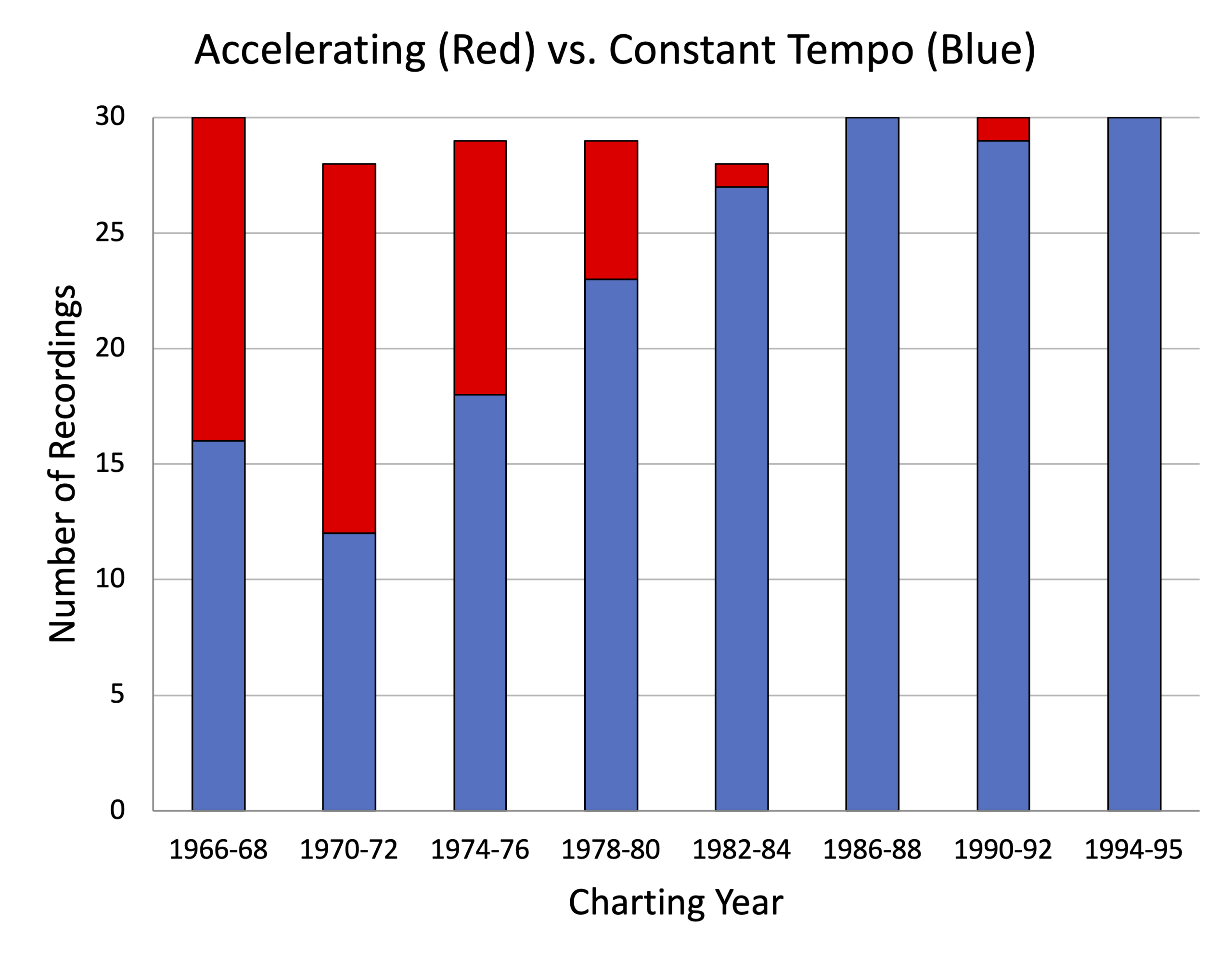
Building on the work of Roessner and Condit-Schultz and Clark but using our original method, we examined with greater specificity the trend toward the use of click tracks in mainstream popular music. Shown in Figure 4, yearly median CV values40 exhibit a mostly consistent downward trend, from a corpus high of 1.51 in 1972 to a low of 0.03 in 1994.41 Appendix Table 3 shows the median, mean, and standard deviation for each year studied, as well as values excluding ritardandi and tempo shifts. From 1982 on, the median values are always below 0.5, the approximate dividing line between unaided playing and use of a click track, drum machine, or sequencing. And the decline in tempo variability can be observed in other ways. Figure 5 shows that significant acceleration over the course of a song became much less common over this same time frame. The figure compares the number of songs in given years of the Billboard tempo corpus that accelerate with those maintaining a relatively steady tempo. In this graph, recordings are considered to be “accelerating” if the tempo of the final two measures (excluding closing ritardandi) is at least 3% higher than that of their first two measures, while recordings are considered to have a “constant” tempo if there is less than a 3% difference between the tempo of their first two measures and that of their last two. The evidence suggests that both intentional, expressive tempo alterations as well as gradual, unintentional tempo variability became less common in the popular mainstream after the 1970s.42
The data between 1976 and 1979 reflects major changes that occurred in music production during that time period. 1976 was the first year in the Billboard tempo corpus containing any songs with tempo CVs lower than 0.5, the timekeeping assistance threshold: Gary Wright’s funky “Love Is Alive” (CV = 0.21; released in 1975), which used a drum machine as a click, and Silver Convention’s disco hit “Fly, Robin, Fly” (1976, CV = 0.21),43 featuring drummer Keith Forsey playing to a Wurlitzer Side Man drum machine (Shapiro 2005, 93). In 1978, three of the year-end top 15 songs had CV values less than 0.5: the Bee Gees’ “Night Fever” and “Stayin’ Alive,” both from the 1977 Saturday Night Fever soundtrack, and John Travolta and Olivia Newton-John’s “You’re the One that I Want.” Nevertheless, the other twelve of the year-end top 15 songs had tempo CVs over 0.5, indicating a lack of use of click tracks or other timekeeping assistance. But in 1979, ten of the top 15 hits, many of them disco songs, had tempo CVs under 0.5.44 Figure 6 shows the trajectory over this time period toward an increasing number of songs recorded to a click, with a particularly large jump going from 1978 to 1979. The median tempo CV for 1979, 0.46, is substantially lower than that for 1978 or any preceding year in the corpus and the first under the 0.50 threshold. Appendix Table 4 shows all Billboard tempo corpus songs from prior to 1980 with CV values less than 0.5, along with the best available information as to the timekeeping mechanism used.
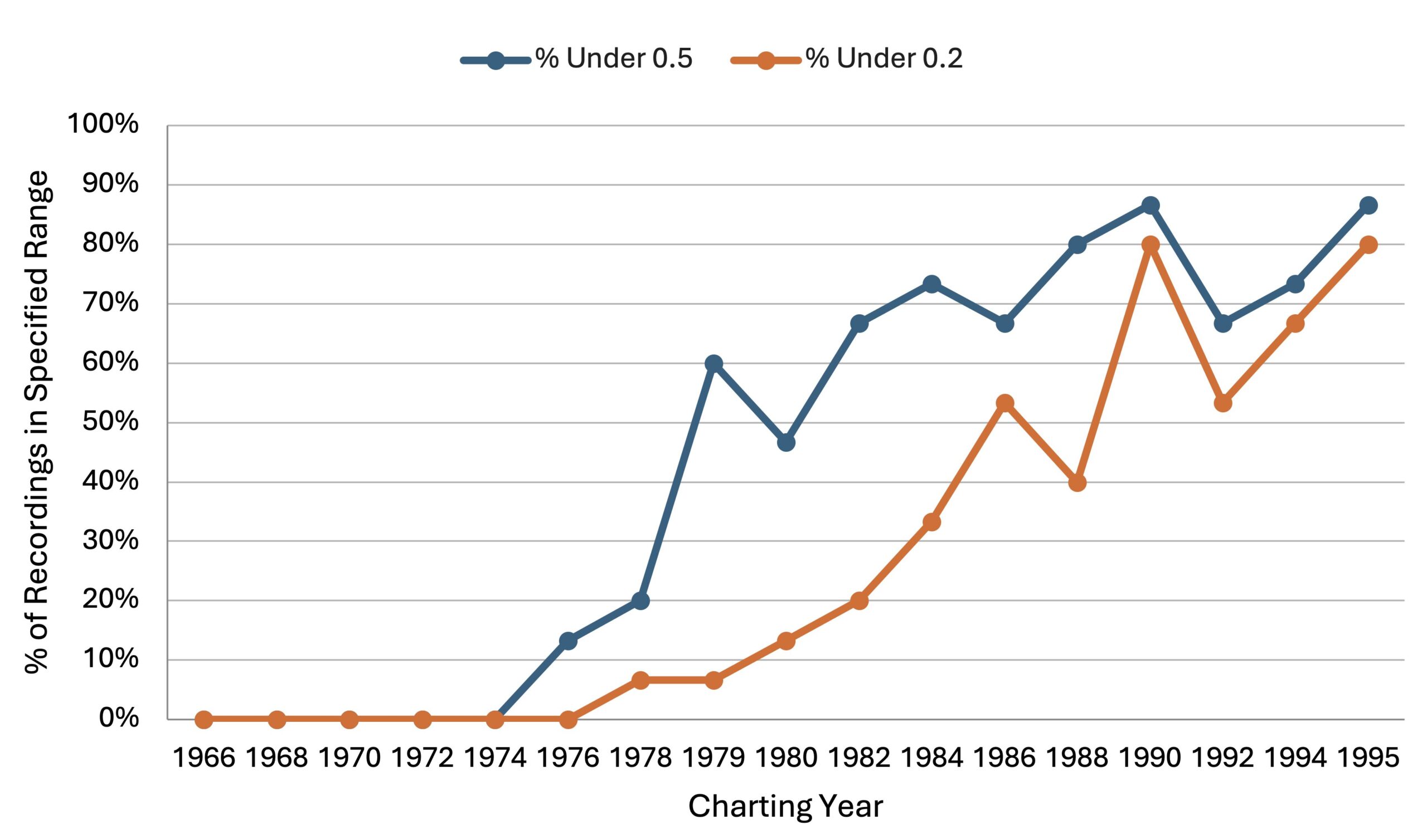
In 1980, in the wake of disco’s demise, the median CV rebounded slightly to 0.65—higher than 1979 but still lower than any of the median values prior to that year. Notably, the 1980 year-end chart included a few songs that can be considered pre-disco-era throwbacks, including Queen’s AABA-form “Crazy Little Thing Called Love” (CV = 1.29), a rockabilly pastiche, and Billy Joel’s AABA “It’s Still Rock and Roll to Me” (CV = 1.73), a paean to the primacy of the music of Joel’s childhood (Example 7 and Video Example 7 above).45 Afterward, the median tempo CV in 1982 descended again under the 0.5 line to a new low of 0.44 and remained below that threshold through the end of our study. 1982 is the first year in the Billboard tempo corpus with songs featuring a sounding drum machine, including the Human League’s new wave “Don’t You Want Me” (CV = 0.02), in which an LM-1 was controlled by a Roland MC-8 sequencer (LeRoy 2023, 146–148). 1986 was the earliest year we analyzed where the median CV, 0.18, was within the range indicating a sounding drum machine or sequence. The median CV for 1994, 0.03, is the lowest of any year that we analyzed, reaching a nadir of variability that was nearly matched by 1995’s median of 0.08. By 1994, sequencing technology had almost completely taken over the percussion and drums in the biggest Billboard hit singles, with nearly perfect metronomic regularity prized over the imperfections of human drumming.46
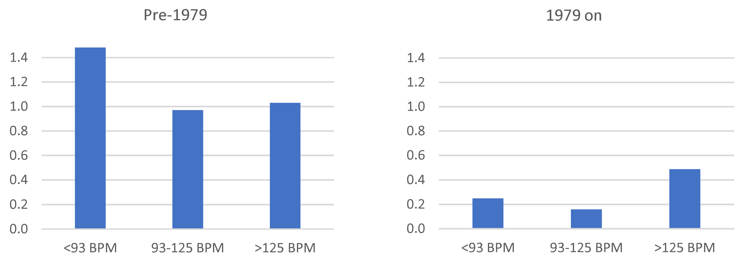
Another prominent factor affecting the CV values in the Billboard corpus is their tempo. Slower songs that charted prior to 1979 tend to have greater tempo variability.As seen in Figure 7,47 the median CV value for pre-1979 corpus songs with tempi less than 93 BPM was 1.48, significantly higher than that for mid-tempo (0.97) or fast (1.03) songs.48 Barbra Streisand’s “The Way We Were” (1974), seen in Example 21, exemplifies the appearance of many 1970s ballad tempo maps. From 1979 on, however, slower songs such as Robert John’s “Sad Eyes” (1979) and Phil Collins’s “Against All Odds” (1984) tended to be metronomically steady for most of their duration, with 1980’s “The Rose” being a notable exception. Table 6 shows a selection of ballads in the Billboard tempo corpus along with their CV values. In songs charting from 1979 on, the median CV was 0.26 for slow songs, 0.16 for mid-tempo, and 0.49 for fast recordings. In this latter period, the fast songs have the most variability, with a number of these recordings being upbeat rock throwbacks recorded without a click track, such as Guns N’ Roses’ “Sweet Child O’ Mine” (1988), Van Halen’s “Jump” (1984), and “It’s Still Rock and Roll to Me.” Both before and after 1979, mid-tempo songs had the lowest CV values. This tendency may result in part from how dance music (including disco) inclines towards both moderate tempi (Moelants 2003, 649) and low tempo variability.
| Song | Artist | Year | Mean Tempo | CV w/o Rit. | Full CV |
|---|---|---|---|---|---|
| Strangers in the Night | Frank Sinatra | 1966 | 90 | 8.98 | 8.98 |
| Let It Be | The Beatles | 1970 | 71 | 3.39 | 3.46 |
| The First Time Ever I Saw Your Face | Roberta Flack | 1972 | 61 | 2.84 | 4.83 |
| Without You | Nilsson | 1972 | 65 | 1.94 | 1.94 |
| The Way We Were | Barbra Streisand | 1974 | 66 | 5.83 | 9.76 |
| You Light Up My Life | Debby Boone | 1978 | 76 | 2.40 | 9.09 |
| Sad Eyes | Robert John | 1979 | 71 | 0.24 | 0.24 |
| The Rose | Bette Midler | 1980 | 64 | 3.59 | 5.36 |
| Against All Odds | Phil Collins | 1984 | 58 | 0.14 | 2.25 |
| Friends And Lovers | Carl Anderson and Gloria Loring | 1986 | 36 | 0.52 | 3.63 |
| Anything For You | Gloria Estefan | 1988 | 72 | 0.32 | 0.32 |
Table 6. Selected ballads from the Billboard tempo corpus and their tempo CVs. “CV w/o Rit.” excludes a closing ritardando.
8. Conclusion
Our original methodology of combining automated tempo analysis with manual adjustments allows for the examination of patterns of tempo variability; for detection of whether a click track, drum machine, or sequencing was used; for the close analysis of individual songs; and for the detection of long-term trends. Worthy of study are clearly audible tempo shifts, the subtler changes that happen when no timekeeping assistance is used, the greatly decreased tempo variability when a click track is employed, and the hybrid situations in which timekeeping assistance is used in combination with passages without it. While tempo in pop music is often conceptualized as steady and not worthy of close analysis, our paper suggests that approaches to tempo variability have changed over time, and understanding how it functions in a particular case is a crucial component to analyzing a recording. Individual songs, such as “The Rose” and “I Will Survive,” exist within the context of larger historical trends.
Going forward, our method could be used to examine patterns and calculate tempo CVs for larger numbers of songs in order to determine more precisely how tempo variability changed over time. In particular, analyses could be made both of recordings stretching back into earlier decades as well as of more recent music, to see whether the trend toward tempo invariability has continued to the present day. Further analysis could help determine how genre correlates with patterns and degree of tempo variability, looking at country, rock, metal, hip-hop, and R&B. Tempo CV could even be used to assist in automatic identification of genre. The extent of correlation between tempo CV and lyrical content, mode, or instrumentation could also be examined (see Zicari 2017, 51–52; connecting tempo variability in opera recordings with the lyrical content), as well as the timing profiles of particular drum machines. Finally, it would be valuable to study the cultural implications of timekeeping technology—to determine whether different generations of listeners vary in their aesthetic responses to tempo invariance as well as how steadiness and variability have acted as opposing forces over the history of popular music. Tempo variability and historical changes in approaches to it will be particularly worthy of attention because they are often not consciously recognized by listeners, exercising a fundamental but hidden influence on our perception.
The authors would like to thank their assistants Alexis Cantelme, Jonas Kastenhuber, Mira Perusich, and Thomas Zaterka.
References
Amendola, Billy. 2007. “James Gadson: R&B Sound Legend.” Modern Drummer, September 2007, 112–118.
Arachchige, Chandima N.P.G., Luke A. Prendergast, and Robert G. Staudte. 2020. “Robust Analogs to the Coefficient of Variation.” Journal of Applied Statistics 49 (2): 268–290.
Ashley, Richard. 2002. “Do[n’t] Change a Hair for Me: The Art of Jazz Rubato.” Music Perception 19 (3): 311–332.
———. 2014. “Expressiveness in Funk.” In Expressiveness in Music Performance: Empirical Approaches Across Styles and Cultures, edited by Dorottya Fabian, Renee Timmers, and Emery Schubert, 154–169. New York: Oxford University Press.
Attas, Robin. 2015. “Form as Process: The Buildup Introduction in Popular Music.” Music Theory Spectrum 37 (2): 275–296.
Benadon, Fernando. 2006. “Slicing the Beat: Jazz Eighth-Notes as Expressive Microrhythm.” Ethnomusicology 50 (1): 73–98.
Bennett, Samantha. 2019. Modern Records, Maverick Methods: Technology and Process in Popular Music Record Production 1978–2000. Annapolis: Bloomsbury.
Böck, Sebastian, Matthew E. P. Davies, and Peter Knees. 2019. “Multi-Task Learning of Tempo and Beat: Learning One to Improve the Other.” In Proceedings of the International Society for Music Information Retrieval Conference (ISMIR), edited by Arthur Flexer, Geoffroy Peeters, Julián Urbano, and Anja Volk, 486–493. Delft, the Netherlands.
Brøvig-Hanssen, Ragnhild, and Anne Danielsen. 2016. Digital Signatures: The Impact of Digitization on Popular Music Sound. Cambridge, MA: MIT Press.
Brumm, Henrik. 2012. “Biomusic and Popular Culture: The Use of Animal Sounds in the Music of the Beatles.” Journal of Popular Music Studies 24 (1): 25–38.
Bryon, Dennis. 2015. You Should Be Dancing: My Life with the Bee Gees. Toronto: ECW Press.
Buskin, Richard. 2004a. “Classic Tracks: Tina Turner ‘What’s Love Got to Do with It?’” Sound on Sound, May 2004. https://www.soundonsound.com/techniques/classic-tracks-tina-turner-whats-love-got-do-it.
———. 2004b. “Classic Tracks: The Police ‘Every Breath You Take.’” Sound on Sound, March 2004. https://www.soundonsound.com/techniques/classic-tracks-police-every-breath-you-take.
———. 2005. “Classic Tracks: Chic ‘Le Freak.’” Sound on Sound, April 2005. https://www.soundonsound.com/techniques/classic-tracks-chic-le-freak.
Carter, David S., and Ralf von Appen. 2025. “Measuring the Myth: Microtiming and Tempo Variability in the Music of the Rolling Stones.” Theory and Practice 49–50: 91–158.
Coffman, Tim. 2023. “The Classic Nirvana Song That Forced Dave Grohl to Use a Click Track.” Far Out Magazine, 13 May 2023. https://faroutmagazine.co.uk/the-classic-nirvana-song-that-forced-dave-grohl-to-use-a-click-track/.
Collier, Geoffrey L., and James Lincoln Collier. 1994. “An Exploration of the Use of Tempo in Jazz.” Music Perception 11 (3): 219–242.
Condit-Schultz, Nathaniel. 2019. “Deconstructing the nPVI: A Methodological Critique of the Normalized Pairwise Variability Index as Applied to Music.” Music Perception: An Interdisciplinary Journal 36 (3): 300–313.
Condit-Schultz, Nathaniel, and Beach Clark. 2024. “Have We Sold Our Souls to The Drum Machine? A Historical Analysis of Tempo Stability in Western Music Recordings.” Musicae Scientiae 28 (3): 451–477.
Covach, John. 2009. What’s That Sound?: An Introduction to Rock and Its History. 2nd ed. New York: W. W. Norton.
Dahl, Sofia, and Svante Granqvist. 2003. “Looking at Perception of Continuous Tempo Drift: A New Method for Estimating Internal Drift and Just Noticeable Difference.” In Proceedings of the Stockholm Music Acoustics Conference (SMAC 03), vol. 2, 595–598.
Daniele, Joseph R. 2016. “A Tool for the Quantitative Anthropology of Music: Use of the nPVI Equation to Analyze Rhythmic Variability Within Long-Term Historical Patterns in Music.” Empirical Musicology Review 11 (2): 228–233.
DeChristopher, John. 2021. “E29: Live from My Drum Room with Andy Newmark! 3-28-21.” YouTube video, 2:02:09. 28 March 2021. https://www.youtube.com/watch?v=cUQftJ6IFVs.
de Clercq, Trevor. 2012. “Sections and Successions in Successful Songs: A Prototype Approach to Form in Rock Music.” PhD diss., Eastman School of Music.
———. 2016. “Measuring a Measure: Absolute Time as a Factor for Determining Bar Lengths and Meter in Pop/Rock Music.” Music Theory Online 22 (3). https://mtosmt.org/issues/mto.16.22.3/mto.16.22.3.declercq.php.
Demos, Alexander P., Tânia Lisboa, Kristen T. Begosh, Topher Logan, and Roger Chaffin. 2020. “A Longitudinal Study of the Development of Expressive Timing.” Psychology of Music 48 (1): 50–66.
Demos, Alexander P., Tânia Lisboa, and Roger Chaffin. 2016. “Flexibility of Expressive Timing in Repeated Musical Performances.” Frontiers in Psychology 7: 1490. https://doi.org/10.3389/fpsyg.2016.01490.
di Perna, Alan. 1993. “Brian’s Song.” Guitar World, January 1993. http://pages.swcp.com/~unicorn/bri_gw93.txt.
Ellis, Robert J., Zhiyan Duan, and Ye Wang. 2014. “Quantifying Auditory Temporal Stability in a Large Database of Recorded Music.” PLOS One 9 (12): e110452. https://doi.org/10.1371/journal.pone.0110452.
Fabian, Dorottya. 2014. “Commercial Sound Recordings and Trends in Expressive Music Performance: Why Should Experimental Researchers Pay Attention.” In Expressiveness in Music Performance: Empirical Approaches Across Styles and Cultures, edited by Dorottya Fabian, Renee Timmers, and Emery Schubert, 58–79. New York: Oxford University Press.
Flans, Robin. 2004. “Classic Tracks: ‘Every Breath You Take’: The Police.” Mix Magazine, March 2004. https://www.soundonsound.com/techniques/classic-tracks-police-every-breath-you-take.
Friberg, Anders, and Andreas Sundström. 2002. “Swing Ratios and Ensemble Timing in Jazz Performance: Evidence for a Common Rhythmic Pattern.” Music Perception 19 (3): 333–349.
Friedman, Ronald S. 2018. “Final Ritardandi and the Expression of Musical Emotion.” Music Perception: An Interdisciplinary Journal 36 (1): 53–59.
Geary, David. 2024. “Formal Functions of Drum Patterns in Post-Millennial Pop Songs, 2012–2021.” Music Theory Online 30 (2). https://mtosmt.org/issues/mto.24.30.2/mto.24.30.2.geary.html.
Getty, David J. 1975. “Discrimination of Short Temporal Intervals: A Comparison of Two Models.” Perception and Psychophysics 18 (1): 1–8.
Gracyk, Theodore. 1996. Rhythm and Noise: An Aesthetics of Rock. Durham, NC: Duke University Press.
Heath, Harold. 2017. “Gear Tribute: The Maestro Rhythm King MRK–2, Sly Stone’s Favorite Drum Machine.” Reverb, 5 June 2017. https://reverb.com/news/gear-tribute-the-maestro-rhythm-king-mrk2-sly-stones-favorite-drum-machine.
Hesselink, Nathan. 2023. Finding the Beat: Entrainment, Rhythmic Play, and Social Meaning in Rock Music. New York: Bloomsbury.
Inglis, Sam. 2003. “Producer: Steve Levine: Restoring Culture Club’s Back Catalogue.” Sound on Sound, March 2003. https://www.soundonsound.com/people/producer-steve-levine.
Kocher, Philippe. 2023. Dirigierende Maschinen: Musik mit technikgestützter Tempovermittlung. Bielefeld: transcript Verlag.
Kristofferson, Alfred B. 1980. “A Quantal Step Function in Duration Discrimination.” Perception and Psychophysics 27: 300–306.
Lamere, Paul. 2009. “In Search of the Click Track.” Music Machinery.WordPress.com, 2 March 2009. https://musicmachinery.com/2009/03/02/in-search-of-the-click-track/.
———. 2010. “Revisiting the Click Track.” Music Machinery.WordPress.com, 8 February 2010. https://musicmachinery.com/2010/02/08/revisiting-the-click-track/.
LeRoy, Dan. 2023. Dancing to the Drum Machine: How Electronic Percussion Conquered the World. New York: Bloomsbury.
London, Justin. 2001. “Tempo (i).” Grove Music Online. https://www-oxfordmusiconline-com.lmu.idm.oclc.org/grovemusic/view/10.1093/gmo/9781561592630.001.0001/omo-9781561592630-e-0000027649.
MacLeod, Sean. 2024. “When the Earth Becomes a Star: A Songwriter’s Arts Practice Investigation into the Influence of Modern Digital Technology on the Conventions of Popular Music-Making, with an Emphasis on Musical Temperament and Tuning.” PhD diss., University of Limerick.
Madison, Guy. 2001. “Variability in Isochronous Tapping: Higher Order Dependencies as a Function of Intertap Interval.” Journal of Experimental Psychology: Human Perception and Performance 27: 411–422.
———. 2004. “Detection of Linear Temporal Drift in Sound Sequences: Principles and Empirical Evaluation.” Acta Psychologica 117: 95–118.
Madison, Guy, and Bjorn Merker. 2004 “Human Sensorimotor Tracking of Continuous Subliminal Deviations from Isochrony.” National Library of Medicine 370 (1): 69–73.
Milner, Greg. 2009. Perfecting Sound Forever: An Aural History of Recorded Music. New York: Farrar, Straus and Giroux.
Moelants, Dirk. 2003. “Dance Music, Movement and Tempo Preferences.” In Proceedings of the 5th Triennial ESCOM Conference, 649–652. Hanover University of Music and Drama.
Müller, Meinard. 2021. Fundamentals of Music Processing: Using Python and Jupyter Notebooks, 2nd ed. Berlin: Springer Nature.
Mynett, Mark, and Jonathan P. Wakefield. 2009. “The Use of Click Tracks for Drum Production within the Extreme Metal Genre.” Paper presented at The Art of Record Production Conference, Cardiff, Wales, 13–15 November 2009. https://eprints.hud.ac.uk/id/eprint/9164/.
News Coldplay. 2017. “Will Champion Teaching a Masterclass for Rhythm Studios.” YouTube video, 1:33:40. 17 October 2017. https://www.youtube.com/watch?v=uUqRtHvHrZI.
Polfreman, Richard. 2013. “Comparing Onset Detection & Perceptual Attack Time.” In Proceedings of the 14th International Society for Music Information Retrieval Conference (ISMIR 2013), edited by Alceu de Souza Britto Junior, Fabien Gouyon, and Simon Dixon, 523–528.
Pouliot, Marc, and Simon Grondin. 2005. “A Response-Time Approach for Estimating Sensitivity to Auditory Tempo Changes.” Music Perception: An Interdisciplinary Journal 22 (3), 389–399.
Repp, Bruno H. 1992. “Diversity and Commonality in Music Performance: An Analysis of Timing Microstructure in Schumann’s ‘Träumerei.’” The Journal of the Acoustical Society of America 92 (5): 2546–2568.
———. 1998. “A Microcosm of Musical Expression. I. Quantitative Analysis of Pianists’ Timing in the Initial Measures of Chopin’s Etude in E Major.” Journal of the Acoustical Society of America, 104 (2): 1085–1100.
Roessner, Stephen F. 2017. “The Beat Goes Static: A Tempo Analysis of U.S. Billboard Hot 100 #1 Songs From 1955–2015.” In Proceedings of the Audio Engineering Society Convention 143, edited by Areti Andreopoulou and Braxton Boren. Audio Engineering Society.
Ryan, Kevin, and Brian Kehew. 2006. Recording the Beatles: The Studio Equipment and Techniques Used to Create Their Classic Albums. Houston: Curvebender Publishing.
Sagesser, Marcel. 2021. “Within the Grid: Inquiries in the Socio-Rhythmic Ambiguities of Mechanical Time.” PhD diss., Brown University.
Schreiber, Hendrik. 2020. “Data-Driven Approaches for Tempo and Key Estimation of Music Recordings.” PhD diss., Friedrich-Alexander-Universität Erlangen-Nürnberg.
Sclar, Doug. 2019. “Richard Harris’s Version of Jimmy Webb’s ‘MacArthur Park,’ What’s Your Opinion of It?” Forum post, Steve Hoffman Music Forums, 23 August 2019. https://forums.stevehoffman.tv/threads/richard-harriss-version-of-jimmy-webbs-macarthur-park-whats-your-opinion-of-it.868066/page-8.
Shapiro, Peter.2005. Turn the Beat Around: The Secret History of Disco. London: Faber & Faber.
Shea, Nicholas, Lindsey Reymore, Christopher Wm. White, Ben Duinker, Leigh VanHandel, Matthew Zeller, and Nicole Biamonte. 2024. “Diversity in Music Corpus Studies.” Music Theory Online 30 (1). https://mtosmt.org/issues/mto.24.30.1/mto.24.30.1.shea_et_al.html.
Stewart, Jon. 2011. “Jon Stewart with Dave Grohl, Krist Novoselic and Butch Vig // SiriusXM // Lithium.” YouTube video, 3:19. 28 September 2011. https://www.youtube.com/watch?v=js_A2Tg_4h0.
Summach, Jay. 2011. “The Structure, Function, and Genesis of the Prechorus.” Music Theory Online 17 (3). https://mtosmt.org/issues/mto.11.17.3/mto.11.17.3.summach.html.
———. 2012. “Form in Top-20 Rock Music, 1955–89.” PhD diss., University of North Texas.
Sykes, Charles E. 1992. “A Conceptual Model for Analyzing Rhythmic Structure in African-American Popular Music.” Ed.D. diss., Indiana University.
Temperley, David. 2004. “Communicative Pressure and the Evolution of Musical Styles.” Music Perception 21 (3): 313–337.
Théberge, Paul. 2016. “Click / Beat / Body: Thoughts on the Materiality of Time and Tempo.” In The Auditory Culture Reader, edited by Michael Bull and Les Back, 341–348. New York: Bloomsbury.
Timmers, Renee. 2007. “Vocal Expression in Recorded Performances of Schubert Songs.” Musicae Scientiae 11 (2): 237–268.
Todd, Neil. 1985. “A Model of Expressive Timing in Tonal Music.” Music Perception 3 (1): 33–51.
Vukovics, Katherine, and Daniel Shanahan. 2020. “Rhythmic Variability, Language, and Style: A Replication and Extension of nPVI findings with the RISM dataset.” Journal of New Music Research 49 (3): 285–297.
White, Christopher William, Joe Pater, and Mara Breen. 2022. “A Comparative Analysis of Melodic Rhythm in Two Corpora of American Popular Music.” Journal of Mathematics and Music 16 (2): 160–182.
Wikane, Christian John. 2022. “Making Her Move: Olivia Newton-John’s ‘Physical’ Phenomenon Revisited.” PopMatters, 9 August 2022. https://www.popmatters.com/olivia-newton-john-physical/2.
Williams, Stuart. 2023. “JR Robinson on the Michael Jackson Rock with You Drum Intro: ‘I Made Sure There Was a Hole That You Could Drive an 18-Wheeler Through.’” Music Radar, 3 March 2023. https://www.musicradar.com/news/story-of-michael-jackson-rock-with-you-drum-intro-jr-robinson.
Wolf, Thomas, and Günther Knoblich. 2022. “Joint Rushing Alters Internal Timekeeping in Non-Musicians and Musicians.” Scientific Reports 12 (1): 1190.
Zak, Albin. 2001. The Poetics of Rock: Cutting Tracks, Making Records. Berkeley: University of California Press.
———. 2019. “Moving at High Speed into the Future: Notes on British Postpunk Record Production.” In The Art of Record Production, 2nd ed., edited by Simon Zagorski-Thomas, Katia Isakoff, Serge Lacasse, and Sophie Stevance, 38–49. London: Routledge.
Zicari, Massimo. 2017. “Expressive Tempo Modifications in Adelina Patti’s Recordings: An Integrated Approach.” Empirical Musicology Review 12 (1–2): 42–56.
Appendix
Appendix Table 1. Data for the Billboard tempo corpus. If two values are listed in the CV column, the first refers to the calculation for the full song. If not otherwise noted, the second value is the calculation excluding a final ritardando.
* = excluding slower instrumental section at the end;
** = excluding slower introduction;
*** = only the longest section from 1:28 to 6:28;
**** = Part A (0:00–1:10): 1.28; Part B (1:10–3:49): 1.62;
+ = excluding the unsteady intro (0:00–0:22);
++ = Part A (0:00–1:06): .66, Part B (1:07–3:55): .18;
+++ = excluding faster bridge (2:48–3:05) and final ritardando.
Appendix Table 2. Tempo CV and mean tempo values for the supplemental corpus. All Tempo CV values exclude final ritardandi. Years listed are years of release.
Appendix Table 3. Statistical evaluation of the tempo coefficient of variation values for each year in the Billboard tempo corpus. The “Alt.” values encompass calculations that exclude closing ritardandi and measure the majority, steadiest portions of recordings in cases where there is more than one distinct tempo in a song. Values in red are the highest values for a given column; values in green are the lowest.
Appendix Table 4. All songs in the Billboard tempo corpus prior to 1980 with tempo coefficient of variation values less than 0.50, out of 120 total pre-1980 recordings. “Year” represents charting year and not necessarily the year of release.
Notes
- Musical speed or pacing. Tempo is tightly connected with pulse and meter and involves the entire metric hierarchy (London 2001).
- Because there can be ambiguity as to whether a tempo change is discrete or continuous, the distinction between “shift” and “drift” can break down. It can be better to understand tempo changes as a matter of degree—a sliding scale. The Beach Boys’ “I Get Around” (Section 3.4 and Example 10 below) is an example of a song where some tempo changes might be interpreted as either drift or a shift.
- Roessner (2017, 3) points out, however, that using MIRtempo resulted in erroneous analyses of songs where there is a relatively steady beat but no drums.
- Algorithms have more difficulty with non-percussive attacks because such attacks are more gradual and there is no abrupt energy increase.
- See also Lamere (2009, 2010) regarding detection of click track usage. Lamere’s approach primarily relied on a subjective visual assessment of tempo deviation graphs, though he did introduce two single-number metrics in his 2010 post that can be thought of as predecessors to our use of tempo CV (see Section 4 below).
- In this paper we primarily analyze recordings but sometimes use the term “song” for stylistic reasons, to avoid repetition and aid readability (for more on this distinction see Gracyk 1996, 43).
- Year specifications for songs from this Billboard tempo corpus refer to the charting year and not necessarily the release year. All songs referenced in this paper are from the Billboard tempo corpus unless they have an asterisk next to their year designation, in which case they are part of the supplemental corpus.
- While creating a corpus from a chart that ranks songs based on sales and radio play has the advantage of avoiding the “fan mentality” problem discussed by Covach (2009, 6) and Summach (2011, 5), the use of such charts has the potential to reinforce societal racial or gender bias (Shea et al. 2024, 0.2).
- With the exception of a few purposefully selected live tracks in the second corpus, with both corpora we selected the original version of the song that charted (typically the seven-inch studio-produced single), since numerous songs appear to have later been quantized in the process of being digitally remastered (see footnote 43 below).
- A great deal of literature and industry research has focused on detecting beats and tempo in commercial recordings (see, e.g., Schreiber 2020; Böck, Davies, and Knees 2019). Automatic beat detection uses some combination of four approaches: energy-based, spectral-based, phase-based, and complex-domain (Müller 2021, 311–321). Richard Polfreman (2013, 527–528) evaluated an earlier version of Melodyne and found that it was very effective in marking percussive attacks. Like all automatic onset detectors, it had more trouble with blown and bowed attacks, yet still fared better than competing tools.
- Octave errors occur when the algorithm determines the tempo to be one half or double the actual tempo. Different listeners can sometimes disagree on which octave the tempo is in and there may not be a single “correct” tempo in some cases, but theorists have sought objective means of determining octave. Deciding the length of a measure and thus the correct octave depends on such factors as the kick-snare pattern, duration in seconds, harmonic rhythm, and form (de Clercq 2016; White, Pater, and Breen 2022, 4–5). Our normalization of tempo standard deviation measurements to the mean tempo of a song minimizes the effect of choice of tempo octave. But, because tempo coefficient of variation values (see below) are lower when a longer time span is analyzed for the individual tempo measurements, choice of a lower-tempo octave can slightly affect such calculations. Toto’s “Rosanna” (1982), for example, has a tempo coefficient of variation value of 1.68 when analyzed as at 130 BPM, but a value of 1.61 when counted as at 65 BPM. Temporary shifts to double-time or half-time feels in our analyzed songs were treated as if in normal time rather than as a tempo change.
- Potential alternatives to Melodyne’s tempo detection algorithm did not work as well. Simon Dixon and Chris Cannam’s BeatRoot, available as a plug-in for Sonic Visualiser, is easy to use and produced good results for recordings with steady tempi. But the plug-in often had problems detecting the tempo in sections with ritardandi and sometimes produced tempo octave errors or mistook off-beats for downbeats. Test runs with Python-based “librosa.beat.beat_track” also led to unsatisfying results, such as very improbable tempo and CV values. With both BeatRoot and Librosa, identifying and manually correcting the results is extremely difficult or even impossible, while Melodyne allows for easy adjustments.
- Logic Pro also can also create tempo maps, but we used Melodyne for this task because corrections to maps can be made more easily and reliably with it.
- Using a rhythmic duration, like two measures, rather than a time length, like two seconds, provides a closer connection to the musical structure of the song. We chose two measures rather than one as it better reflects listener perception, which encompasses a longer time span than one measure when developing a sense of the current tempo. See Madison (2004, 101–102; noting a two- to five-second limit for retention of tempo information and providing listeners detecting tempo drift with pulse streams of up to nine beats) and Schreiber (2020, 117, 119; using twelve-second windows to measure tempo stability).
- Previous scholarship that has used the coefficient of variation in order to measure musical tempo variability includes Schreiber (2020, 85–86, 118–119), Zicari (2017, 51–52; operatic arias), Repp (1998, 1088; Chopin étude), and Collier and Collier (1994, 224–225; historical jazz recordings). CV values calculated by different authors cannot necessarily be directly compared, given that they use different spans of time for local tempo measurements. Condit-Schultz and Clark (2024) instead use log-tempo interquartile range, which excludes from consideration half of a song (the top and bottom quartiles of tempo measurements), to measure variability; this approach, however, potentially excludes crucial tempo information, such as ritardandi and accelerandi, that can be contained in the unconsidered portion. Arachchige, Prendergast, and Staudte (2020) discuss the strengths and weaknesses of coefficient of variation as a statistical measure, as well as alternatives like interquartile range.
- We used single-measure tempo measurements for calculating nPVI because the resultant values better coincided with patterns in tempo maps than did using consecutive sets of two measures.
- nPVI has previously been used in music scholarship primarily to compare differences in adjacent durations in notated music (see, e.g., Daniele 2016; Vukovics and Shanahan 2020), yet it can also be used (with arguably greater effectiveness) to compare adjacent tempo values in recordings. Condit-Schultz (2019, 311) critiques the use of nPVI for notated score data and suggests that it can be more useful for measured performance data that eschews rhythmic categories, such as the recordings we study here.
- Ritardandi are distinct from both tempo shifts and tempo drift. Like tempo shifts, they typically involve large tempo changes and are easily noticeable, but they differ from tempo shifts in that (1) they are continuous rather than discrete, and (2) for internal ritardandi in popular music, the tempo typically then returns to its previous speed. Like tempo drift, ritardandi are continuous, but they differ from tempo drift because they involve larger tempo changes and occur within a short span of time.
- Even outside of intros, passages without a drum kit playing tend to be slower. In Archie Bell & the Drells’ 1968 “Tighten Up,” for example, the two-measure breaks where the drums do not play (such as at 1:19) are the slowest parts of the song, while the busy four-measure drum solos (such as at 0:42) are the fastest portions.
- Attas (2015, 278) notes that the tempo both speeds up and becomes more regular once the drums and bass enter as part of the buildup introduction in Nirvana’s “Come as You Are.”
- Alternatively and much more rarely, a sudden shift (rather than a gradual change) to a dramatically slower tempo at the end of a recording can act as a formal culmination, as in Billie Eilish’s 2019* “Bad Guy” (Geary 2024, 4.19).
- Each of these four songs has a tempo CV ranging between 1.75 and 2.55 as well as a nPVI/CV ratio within the relatively narrow range of 0.24 to 0.39. The CV values are thus much lower than those of songs with clearly audible tempo shifts (which tend to be above 6), and the nPVI/CV ratios are higher, though still well below the corpus median ratio of 0.67.
- Collier and Collier (1994, 233), in their study of tempo variability in jazz, similarly found that pianist Teddy Wilson showed a mostly consistent tendency to play the bridges of songs at a slightly faster tempo than the A sections.
- A drum machine could also be used as a click to allow for slightly different tempi in different sections. According to Jeff Porcaro’s brother Steve, Jeff overdubbed live drums on tempo maps created with a drum machine in the mid-1970s on Seals and Crofts tracks, using slightly faster tempi for choruses (LeRoy 2023, 132). Programming marginally contrasting tempi for different sections seems even more common in the twenty-first century. Olivia Rodrigo’s “Good 4 U,” for example (2021*, CV = 0.88, MnPC = 0.20), has verses at 169 BPM, slightly faster than the choruses at 166 BPM. For Coldplay’s use of tempo maps in the studio, see News Coldplay (2017, 5:30–6:15). See also footnote 35 below.
- Figures in Tables 3a and 3b exclude any closing ritardando, and songs with an abrupt and clear tempo shift are not included.
- See, for example, the officially released versions on Love You Live (recorded 1976, with a tempo increase from 105 to 123 BPM) and Some Girls Live in Texas (recorded 1978, from 103 to 124 BPM). See also Carter and von Appen (2025, 118–120, 125).
- While “Honky Tonk Women,” like songs with large tempo shifts such as “Love Hangover,” features a relatively high tempo CV (3.49) combined with a low nPVI/CV ratio (0.15), its largest individual nPC is only 1.87 because the acceleration is gradual. By comparison, the maximum nPC in “Love Hangover” is 26.06, occurring at 1:11 in the song.
- Examples from outside the Billboard tempo corpus that slow down significantly include the Beatles’ “Michelle,” “Rain,” “I Want to Hold Your Hand,” “She Loves You,” “A Hard Day’s Night,” “You Really Got a Hold on Me,” and “It Won’t Be Long.”
- For example, Albin Zak’s 2001 monograph The Poetics of Rock: Cutting Tracks, Making Records, which examines in great detail the process of rock music production, has only three brief references to click tracks, despite their having been a crucial part of most mainstream rock recordings since 1979. Producer John Leckie in a 1992 interview in this book refers to click tracks as one of “the worst things invented in the last ten years” (Zak 2001, 61). Lamere (2009) claimed an even later date for the rise of click tracks in rock drumming, writing that they came to prominence “sometime in the last 10 or 20 years.”
- As an example, musicologist Samantha Bennett writes in her 2019 book Modern Records, Maverick Methods that no click track was employed for U2’s “Where the Streets Have No Name” (1987), arguing that going without one reflected the band’s bucking of contemporary trends by using older, outdated approaches to production (2019, 49–50). Yet calculating the tempo CV for the entire song starting with the second measure after the entry of the drums gives a value of 0.20, which unambiguously shows the use of timekeeping assistance (see below). As another example, the Beatles’ “Blackbird” includes a tapping sound that many listeners over the years, including scholars, have thought was a metronome (see, e.g., Brumm 2012, 31). But the recording has a tempo CV of 1.40, consistent with engineer Geoff Emerick’s recollection that the sound was in fact Paul McCartney’s foot tapping (Ryan and Kehew 2006, 484).
- Use of a click track can be a source of shame for a drummer. Nirvana’s Dave Grohl, speaking twenty years after the release of Nevermind, said of being asked by producer Butch Vig to play with a click on the album’s “Lithium” (1991*): “The first time a drummer hears that the producer wants them to work with a click track, it’s like getting stabbed in the heart with a rusty fork” (Stewart 2011, 1:34–1:48).
- The term “click track” can either refer to use of a dedicated click to guide a drummer, like a UREI 962 or 964 digital metronome, or can refer to using a drum machine (that is not heard on the recording) as a metronome for the same purpose.
- We also identified a few instances where a click track was used but the tempo CV was slightly under 0.2: this was true of “I Will Survive” (0.16 excluding the freer intro; see Section 6) and “MacArthur Park” (0.18 for the disco portion).
- Songs with values between 0.25 and 0.30 in most cases used a click, though many, such as Chuck Berry’s “Roll Over Beethoven” (0.28), did not. Occasionally a song that relied on a click will have an MnPC value in the 0.30–0.40 range, though this range usually indicates a lack of metronomic assistance.
- Additionally, if slightly different tempi have been programmed for different sections of a recording, the tempo CV may be above 0.50 but the MnPC will reveal use of sequencing. Chris de Burgh’s “The Lady in Red” (1986*), for example, which contains two extremely steady tempi separated by 1 BPM (see Section 3.4 above), has a tempo CV of 0.54 but an MnPC of 0.05.
- Marcel Sagesser (2021, 46–62) engages in a detailed analysis of the interaction between overdubbing drummer Andy Newmark and a Maestro Rhythm King MRK-2 on Sly and the Family Stone’s 1973 “In Time,” arguing that the relationship between the drummer and the machine was a symbiotic collaboration that gave rise to a “synchronous organism” (60).
- Timmers similarly found a tendency to slow the tempo at moments of high tension in recordings of Schubert songs (2007, 253).
- Tempo CV is very sensitive to outlier values, and if one were to interpret this pause on the dominant at 2:32–2:38 as a single measure with a tempo of 38.9 BPM (the rather arbitrary value if we make manual adjustments to the Melodyne map in order to attempt to reflect a possible pulse), then the tempo CV for the song would be 7.52, higher even than that of “The Rose.”
- In this way the silent, hidden metronome exercises authority over even the apparent deviation from isochrony. Similar “simulations” of anisochrony occur in Lionel Richie’s “Say You, Say Me” at 2:51 (three beats of the click track pulse) and in The J. Geils Band’s “Centerfold” at 2:42 (nine beats of the click track pulse). Singer-songwriter Harry Middlebrooks, active in the Los Angeles music scene in the 1970s and ‘80s, says that, when playing with a click and a ritardando was desired, it was common practice to decide ahead of time how many clicks to give the ritardando. This would allow the performers to keep playing to the click while simulating a stretching of time (Middlebrooks in discussion with the authors, 17 July 2024). In Donna Summer’s cover of “MacArthur Park,” the slower introduction is exactly half the speed of the up-tempo disco portion, so the producers could have kept the same click track running through both the ostensibly more expressive introduction and the futuristic remainder. The tempo CV for both the introduction (0.42) and the disco portion (0.18) are under the 0.50 technological assistance threshold.
- We use medians rather than means to minimize the influence of outlier songs.
- Graphing the average MnPC for each year analyzed shows a very similar shape. The increase in variability in both groups in the late 1960s and early 1970s is perhaps consistent with Condit-Schultz and Clark’s (2024, 12, fig. 4) data for the “rock” genre, which shows a marked increase in tempo variability moving from the mid-1960s to the late 1960s.
- The marked uptick in tempo variability Condit-Schultz and Clark (2024, 10, 12, fig. 4) found in rock in the 1990s was not reflected in the median values in our Billboard tempo corpus data. This difference is likely explained by differences in composition of the corpora, with the grunge and “alternative” rock recordings included in Condit-Schultz and Clark’s rock category making relatively little impression on the Billboard year-end top 15. But Figure 6 below reflects some of this influence.
- CV analysis of the remastered versions of tracks like “Fly, Robin, Fly” reveals that many songs with slight amounts of tempo variability have been quantized decades later. While the original seven-inch single of “Fly, Robin, Fly” had a CV of 0.21, the version remastered in 2010 is a completely flat line, with a CV of 0.01. Similarly, the Bee Gees’ “Stayin’ Alive” (1978) originally had a CV of 0.10, but the 2009 remaster has a CV of 0.02. Queen’s “Another One Bites the Dust” (1980*), Donna Summer’s “Bad Girls” (1979), and Prince’s “When Doves Cry” (1984) are additional examples of tracks previously with small amounts of variability whose remastered versions have been quantized. These quantizations are not widely publicized and bring up concerns similar to those discussed by Brøvig-Hanssen and Danielsen (2016, 66–67) and Milner (2009, 220–227) regarding remastering in general, with the process of digitization for release on CD (and later as mp3 or streaming media) ostensibly “perfecting” the previous imperfections of tape and vinyl. Unofficial posts of songs on YouTube sometimes also have been quantized, so it is crucial when doing a CV analysis to use the original recording if an accurate historical assessment is desired. Our method allows for recognition of such retroactive quantization.
- The steep decline in the median tempo CV going from 1978 (0.84) to 1979 (0.46) can be attributed in part to the increased mainstream popularity of disco (Hesselink 2023, 109–110) and particularly to imitation of the Bee Gees’ enormously successful model of metronomically regular dance music, with nine of the 1979 top 15 being disco songs and seven of those nine having CVs indicating use of a click track or loop. The ascendance of drum machines and click tracks in the late 1970s and early 1980s was closely tied to use of a four-on-the-floor kick pattern, a disco mainstay (Zak 2019, 42–43), as well as to the embrace of an aesthetic of artificiality (LeRoy 2023, 95).
- A year later in 1981, Joan Jett & the Blackhearts’ “I Love Rock ‘n Roll” (1982; Example 11 above), with a CV of 1.81, sounded a similar theme of revolt against the metronomic steadiness of the prevailing aesthetic.
- Figure 6 shows a dip in the percentages of corpus songs with low CVs in 1992, bucking the overall upward trend. This dip subtly reflects the rise of “alternative” acts like the Red Hot Chili Peppers, the revival of aging rockers like Eric Clapton, and the incursion into the Hot 100 of country acts like Billy Ray Cyrus. See also footnote 42 above.
- Excluded from Figure 7 are the six Billboard tempo corpus songs that feature (at least) two distinctly contrasting tempi in different tempo categories (“Raindrops Keep Fallin’ on My Head,” “Ain’t No Mountain High Enough,” “American Pie,” “Love Hangover,” “MacArthur Park,” and “Say You, Say Me”).
- This contrasts with Bruno Repp’s (1998, 1088) finding that pianists’ recordings of the beginning of a Chopin étude with slower tempi exhibited slightly lower tempo CVs than those at faster tempi. Our tempo divisions into “slow,” “medium,” and “fast” are based on Sykes (1992, 116), though we used 125 BPM as the cutoff for fast songs rather than 138 in order to ensure there would be enough corpus recordings included in the category to show statistically significant results.